Differential photometry using Canopus
1.0 Introduction
This document summarises the process for
obtaining a light curve from a set of images using differential photometry. In
such a case it is not necessary to determine the magnitude – intensity
relationship. The lessons referred to are those included in the Canopus
Astrometry and Photometry User Guide. Refer to the
When results from several observing runs (or sessions) are to be added together to create a composite light curve work through paragraphs 3 through 6 for the first session and then repeat these actions for the further sessions.
In order to simplify reference to the various lessons, etc. you might like to print them down and keep them in a folder with this document.
Please note that there is much more to Canopus than this particular process – the package includes facilities for both astrometry and photometry (differential and all-sky).
2.0 Setting
the configuration (Lesson 1)
Open
To import the data in to Excel it would also appear to be necessary to set Plot Method to Range. For asteroid lightcurves uncheck ‘Heliocentric times’ this facility being more relevant for variable stars.
New configurations can be set up by entering a new name in the Profile box, entering the relevant data and clicking on OK.
3.0 Create
a session
3.1 Definition
of a session
A session (as defined on P156 of the
3.2 Creating
a Session (Lesson 11)
Follow the instructions as given in Lesson
11 but entering the data relevant to your observations (ie; object, start
date/time, telescope, focal length, CCD camera, temperature, exposure).
The values inserted automatically in the E(stimated) Mag, E(arth) Dist, S(un) Dist, RA and Dec boxes can be compared with your own data (eg; by plotting the asteroid’s track in Megastar) as a check.
When you click on the Calc button an
Asteroid Look-up window is opened to enable the relevant asteroid to be
selected from the
3.3 Exporting data (for import in to a
spreadsheet such as Excel)
In the Photometry Sessions Data window (Sessions Data tab) click on ‘To file’ and save data as a text file. This saves telescope, camera, etc details as entered in the Session Data window and instrumental magnitudes for comparison stars and asteroid. An average value for the instrumental magnitude of the comparison stars is calculated and listed together with associated Julian dates. For this average value to be calculated it is necessary to select Instrumental and to set Plot Method to Range under the Photometry tab in the Configuration window.
4.0 Setting
apertures
The three combo boxes in the centre of the toolbar are used to set the measuring or star aperture, dead zone (difference between star aperture and inner sky annulus) and sky annulus (outer minus inner radii) respectively.
5.0 Calibrating images
Master Dark and Master Flat images are created using the Batch process tool which is accessed by clicking on Utilities/Image Processing/Batch process. The details are in Help/Contents/Image Processing – Creating a Master Dark and ditto Master Flat respectively and in Help/Contents/ Image Processing/Batch Processing.
To calibrate images;
- access the Batch process form; Utilities/Image Processing/Batch process
- select Action; Merge Dark and Flat
- select Master Dark and Master Flat in relevant boxes (top left of window)
- select images to be calibrated (left middle and bottom windows)
- select Save to directory (or Save in original directory)
- click on Process and image names will be displayed in the lower right hand window as the images are processed (if the Process button is greyed out click on the Merge Dark and Flat in the Action window again).
6.0 Generating
a light curve
If you are unsure as to the position of the asteroid (or to check for other asteroids on the image – discoveries ?!?) use the Blinker as described in Lesson 4. Although the lesson describes opening 2 images it is possible to open several. Check that the ‘gunsight’ is in the correct position on all images to be blinked – I have found that it can move from its original spot as further images are opened.
The relevant session must first be selected. Open the Session window (Photometry/Session) and select the required session by clicking on the session number under the Session Data tab and then on OK.
Use the following lessons in sequence;
Lesson 12; Using the Lightcurve
Wizard
Those of you with equatorial mounts will be pleased
to know that
Lesson 13; Measuring the Images
Paragraph 12 refers to the Photometry Sessions Data window. Note that all Object and Comparison star magnitudes are 99.9 because only instrumental magnitudes are being considered.
Lesson 14; A Quick Peek
Work through this lesson to obtain a light curve.
7.0 Finding
the light curve period
The procedure is described in Lessons 16 and 17. It can be used to analyse results from a single observing session or to combine the results of several. If several sessions are being combined then you must have worked through paragraphs 3 through 6 for each session.
8.0 Saving the data
The light curve, obtained as described in para 6.0,
Lesson 14; A Quick Peek, can be saved by clicking on the printer icon at the
top right hand corner of the screen. These charts take up a lot of disk space,
approx 2 MB, and people without broadband might not be too happy to send and/or
receive them ! A JPG version of the same chart takes up only approx 95 KB and
are thus easier to handle. I convert mine using Graphic Workshop
Professional.
To save the data go to the Observing Sessions form (Photometry/Session), select the required session and click on File. Select the Output Options and JD correction required and click on OK.
9.0 An example
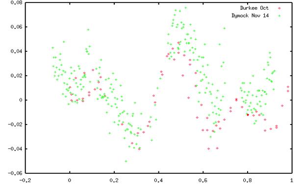
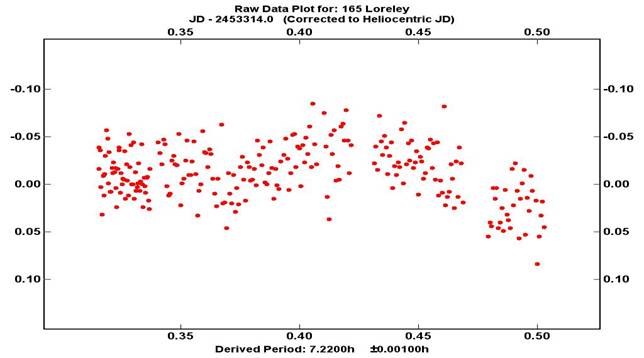
I imaged 165 Loreley on 4th and
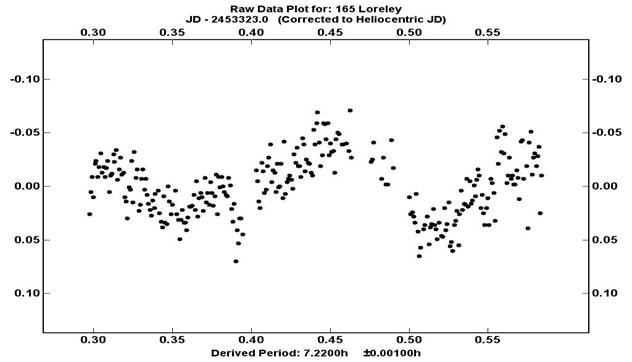
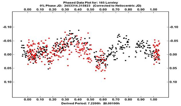
Shown below are three light curves; one for each of the two nights and a combined one using the previously determined period of 7.22 hrs (Astronomy and Astrophysics 197, 327-330 (1988), ‘165 Loreley, one of the last large “unknown” asteroids’ by H.J.Schober, M.Di Martino and A,Cellino).
Please note that the charts below show that the data has been corrected to heliocentric JD. As mentioned earlier this is not necessary for asteroid light curves
4th
November
13th
November
4th
and 13th November data
The response from