Jupiter’s polar polygons:  Circumpolar clusters of cyclones

John H. Rogers [1], Gerald Eichstädt [2], Candice J. Hansen [3], Glenn S. Orton [4], Michael Caplinger [5], Thomas Momary [4], & Fachreddin Tabataba-Vakili [4]

(1) British Astronomical Association, London, UK; (2) Independent scholar, Stuttgart, Germany; (3) Planetary Science Institute, Tucson, Arizona, USA; (4) Jet Propulsion Laboratory, Caltech, California, USA; (5) Malin Space Science Systems, San Diego, California, USA.

8 March 2018

When NASA’s Juno spacecraft, on its first orbit around Jupiter, produced the first clear images of the planet’s poles, they revealed remarkable clusters of cyclones around each pole [ref.1], quite unlike the single giant cyclone that is seen at each pole of Saturn.  These circumpolar cyclones (CPCs) were circular in outline, with obvious spiral structure, quite unlike any large cyclonic features anywhere else on Jupiter.  Their organisation became evident over subsequent perijoves, and is today reported in a paper in ‘Nature’ which combines data from JunoCam (the camera) and JIRAM (the Jovian Infrared Auroral Mapper) [ref.2].  At the south pole, five cyclones form a pentagon around a central cyclone; at the north pole, eight cyclones form a modified octagon or ‘double square’ around a central one.

Here we present more details and animations from the JunoCam images. (A more complete account will be submitted to a professional journal.)  As the vision for JunoCam is for public participation in a planetary mission, JHR and GE have had the privilege of working with the NASA JunoCam team (led by CJH) in processing and analysing these images throughout the mission. This work used polar projection maps produced by GE.  The original images and GE’s processed versions are available on the JunoCam web site (https://www.missionjuno.swri.edu/junocam), and annotated images and maps at each perijove, including polar views that include the CPCs, are on the BAA Jupiter Section web site (https://www.britastro.org/node/7982).

The text is also given here in a PDF:    CPCs_report-re-Nature_JHR-FINAL&FIGS.pdf

Reduced-size figures are shown at the bottom of this report.

The full-size figures are here in a ZIP file:    CPCs_Figures-for-JunoCam-report.zip

Animations of the polar cyclones are here:  https://britastro.org/node/12655

JunoCam can only view what is sunlit, i.e. in daylight, during up to 3 hours as Juno flies over each pole, so it cannot cover all longitudes adequately at a single perijove. Coverage is better in the south than in the north, because the planet’s south pole is currently tilted towards the Sun – by 2.5º in 2016 August (PJ1), increasing to 3.6º in 2018 April-May (the southern summer solstice). Conversely the north pole is in darkness, although the CPCs around it can be seen.

Figure 1 is a south polar view compiled from just two perijoves, aligned with just 4º rotation of one so as to display the pentagon well [Footnote 1]. 

Figure 2 is a comparable north polar view, but compiled from 4 perijoves.  This was necessary because the north pole itself is not in sunlight, and because the spacecraft flies over the north pole at lower altitude so does not usually image the whole disk at that point.

The clusters of circumpolar cyclones (CPCs) were quickly noticed in the JunoCam images from the first perijove (PJ1) on 2016 Aug.27 [ref.1].  But with little more than half the region illuminated, it was not evident whether they formed any pattern.  No data were obtained at PJ2.  The PJ3 images (2016 Dec.11), taken over a wider range of illumination, first suggested that the south polar CPCs formed a pentagon [Footnote 2], and north polar ones possibly an octagon.  With the PJ4 images (2017 Feb.2), covering the hemisphere opposite to PJ1, we were convinced of the south polar pentagon – and had to accept that it is not centred on the pole (Figures 1 & 3).  The PJ4 images also reinforced our confidence that the north polar CPCs formed an unusual octagon, which we call a double square or ‘ditetragon’, as alternate cyclones around the octagon have different aspects, so the whole pattern has four-fold rather than eight-fold symmetry (Figures 2 & 4).  These arrangements have been fully confirmed at PJ5 and the subsequent perijoves.  They were also confirmed by the JIRAM instrument, which made maps not by reflected sunlight, but by thermal infrared emission at 5 microns, covering the entire polar regions at PJ4, and large parts at PJ5 [ref.2].

Arrangement of the CPCs

Figures 3 & 4 show maps of the CPCs compiled from images at some of the perijoves.

In the south, there are five CPCs in a pentagonal arrangement surrounding a sixth, central CPC of similar size. Images taken over ~1-3 hours at each perijove resolve five of the six CPCs, and can sometimes locate all six.  The pentagon of CPCs has its outer edge at 80-82ºS, and is ~18º (21,000 km) in diameter.  (Latitudes given here are planetocentric.)  The individual CPCs have diameters of 5.5-7º latitude (6400-8200 km) and most of them are in contact with each other.  (Diameters given in the Nature paper from the JIRAM maps are smaller as they don’t include the outer fringes.)

In the north, each of the early perijoves revealed only 3 or 4 CPCs clearly, and only the PJ1 images showed the fringe of what JIRAM has now identified as the central north polar cyclone.  As the pole is tilting further into darkness, later perijoves successively show slightly less of the octagon.  The octagon has its outer edge at 80-80.5ºN, and its inner edge at 86ºN.  The individual CPCs have diameters of 4.5-6º latitude (5200-7000 km). It appears from the JunoCam maps that the octagon is centred not far from the pole and is stably maintained with only limited swings to and fro around the pole.

     The north polar CPCs fall into two types which alternate around the octagon. All have outer parts with trailing spiral arms, but they differ in their less patterned inner parts.  One type we call ‘filled’: the inner part is a large, sharply-bounded, lobate area, bright white near the edge but reddish-brown inside, which appears to be a continuous cloud deck except for several dark ‘holes’.  The other type we call ‘chaotic’: in three of these, the inner part consists of small-scale cloud streaks and flecks, whereas in the fourth, it resembles the ‘filled’ CPCs though smaller and less regular.

     In maps from PJ1 to PJ5, the mean angle between chaotic CPCs at a filled CPC was ~151º (±5º), while the mean angle between filled CPCs at a chaotic CPC was ~119º (±6º), consistent with the ditetragonal symmetry. However, variations in these angles indicate that there are small deviations from exact four-fold symmetry. Mean latitudes, from PJ1 to PJ5, were as follows: chaotic CPC, 83.4º (±0.5º);  filled CPC, 82.7º (±0.5º).

At the south pole, the pentagon is not so symmetrical. It is approximately centred on the central cyclone, which is offset from the pole by 1.0º to 2.5º latitude, and this offset has varied cyclically: large at PJ1, small at PJ3 and PJ4, large again at PJ6-PJ8, and small again at PJ9 to PJ11.  The centre was ‘precessing’ around an ellipse with a period of about one year; however, it has always been in a narrow longitude range, [towards L3 ~ 218 (±18º) at PJ1-PJ6].  On the side furthest from the pole, there is a gap between two cyclones in the pentagon, and this gap grew larger over the first 8 perijoves, though it was smaller again at PJ11.  On the opposite side of the pentagon is one of the largest CPCs; and adjacent to this, draped around its low-latitude side, is a long, boomerang-shaped band of haze, mostly outside the pentagon but with its kink overlapping the large CPC. [Footnote 3]

All the CPCs are remarkably stable, in appearance and arrangement, according to the JunoCam images.  The polygons have remained intact, though they drift by a few degrees in longitude from one perijove to the next (irregularly in the north; fairly steadily by ~+1.1º/53d in the south up to PJ6, though by more since then), and individual cyclones wander slightly while maintaining the overall patterns.  Within each cluster, individual cyclones have somewhat different aspects, which have been preserved with little change from PJ1 to PJ9.

Circulation of the CPCs

[Posted herewith are some of Gerald’s best animations of the cyclones.]

The circulations in these cyclones are fast enough (0.1 to 0.3 deg/min) that they can be measured from images taken just 15-30 min apart.  The wind speeds given in [ref.2], measured from JIRAM images at a radius of 1500 km in each CPC, were mostly 55-95 m/s.  From JunoCam images, we obtained similar values, and also found that the angular speeds and wind speeds in many of the CPCs were even faster at shorter radii.  Using polar projection maps from the PJ1, PJ3 and PJ4 images, the angular velocities were measured in concentric annuli in the best-resolved CPCs (Figure 5).  Different classes were analysed separately: southern CPCs,  filled northern CPCs, and chaotic northern CPCs. In every case the angular velocity increased towards the centre, as far inwards as the rotation could be discerned, except in the filled northern CPCs.  Many of the CPCs fit a single exponential curve of angular velocity with radius, but a few southern ones were notably faster, and some northern chaotic CPCs were notably slower. The central southern CPC had typical speeds in its outer spiral parts but its innermost part was one of the most rapidly rotating; at PJ4 it reached the highest angular velocity (0.58 deg/min) and wind speed (up to ~157 m/s), with an implied rotation period of only 10.3 hours.  For most other CPCs, the wind speeds were highest between radii of ~900-1600 km, ranging from ~64-105 km/s.  Thus, the CPCs resemble the largest and strongest terrestrial hurricanes, but are several times larger, with diameters of ~5800-8000 km.

For the northern filled CPCs, the inner bright part does not show a centrally increasing angular velocity: two examples showed a uniform rotation rate over a large span from the edge of the inner bright part inwards.  Indeed, in the largest ones there were signs of inner spiral structure suggesting that the very centre rotated less strongly or even, as observed in at least one case, in the opposite direction, i.e. it was anticyclonic.

Surrounding structures and circulation

In order to understand the dynamical context of the CPCs, we are studying the dynamics of the surrounding regions which are largely filled with chaotic stormy cyclonic patches (FFRs).

By ‘blinking’ polar projection maps of JunoCam images, we find that there is no continuous jet around the perimeter of either CPC polygon. Nor is there any consistent pattern of anticyclonic ovals. Indeed, in the north polar region there are only a few very small anticyclonic ovals.  In the south polar region, at each perijove there are several small anticyclonic white ovals scattered outside the pentagon, and we suspect that some of these can be tracked from PJ1 to PJ6, drifting eastwards around the perimeter of the pentagon, in line with the circulations of the CPCs, but at slow and irregular speeds.

The highest-latitude prograde (eastward) jets previously known, from the Cassini zonal wind profile [ref.4], are at 66.0ºN and 64.0ºS (planetocentric). These jets are clearly shown by blinking of the JunoCam polar maps; but no prograde jets are revealed at higher latitudes, although the circulations of FFRs and CPCs are clearly visible.  In the south, though, there is clear evidence for a retrograde (westward) jet at 71-72ºS [see our posted report on the PJ5 images]: from the patterns of FFRs and AWOs in JunoCam images; from JunoCam and ground-based tracking of white ovals at ~73ºS; and from the Cassini profile (although at a slightly lower latitude).  (However, blinking maps suggests that this jet is strong only within the FFRs, not in the short gaps between them.)  The JunoCam images show no indications of flow patterns between the jet and the CPCs.

Discussion

Jupiter’s polar polygons are quite different in nature from Saturn’s famous north polar hexagon.  At each of Saturn’s poles there is a single giant cyclone extending up from 80º latitude, with peak winds of ~160 m/s at 88ºS and 200 m/s at 88ºN.  A prograde (eastward) jet stream surrounds the north polar cyclone, and is distorted by a six-fold standing wave pattern, so that it has a hexagonal shape. In contrast, each pole on Jupiter has a polygonal cluster of cyclones, but no strong jet stream enclosing the cluster.

It seems remarkable that Jupiter’s CPC polygons are so persistent, despite the furious winds which blow within them, and the buffetting from the chaotic, rapidly changing cyclonic structures around them.  It is not yet clear theoretically how this arrangement can be stable, but previous laboratory modelling has revealed that fluids can form patterns called ‘vortex crystals’, which can closely resemble Jupiter’s polar polygons (Figure 6) [ref.5].  Chaotic turbulence in a rotating fluid can spontaneously self-organise into such close-packed ‘crystals’, and we suspect that this is what happens at Jupiter’s poles. (In an analogous process at lower latitudes on a gas giant planet, chaotic turbulence spontaneously self-organises into alternating eastward and westward jets as we see on Jupiter.) The south polar configuration may be a pentagon rather than a hexagon because of the curvature of the planet; but the north polar configuration is more complex and requires further modelling.

Footnotes

Footnote 1: The ‘south polar view’ released by NASA earlier was an early compilation of views from 3 different perijoves, not precisely aligned in longitude, as shown in Figure 7, so the pentagon of cyclones was not coherently shown in it.

Footnote 2: The pentagon of cyclones is shown in an animated map and composite image posted in 2017 Jan. but only now made open-access: https://www.britastro.org/node/8846.

Footnote 3: This band is visible in the maps for PJ5 and PJ8 in Figure 3, and appears as a bright ‘rocket’ near the terminator in the posted animation from PJ5.

References

1.  Orton GS, Hansen C, Caplinger M, et al.  ‘The first close‐up images of Jupiter’s polar regions: Results from the Juno mission JunoCam instrument’  Geophys. Res. Lett. 44,  4599–4606 (2017).  DOI:10.1002/2016GL072443

2.  Adriani A, Mura A, Orton G, Hansen C, Altieri F, Moriconi ML, Rogers J, Eichstädt G, et al. ‘Clusters of Cyclones Encircling Jupiter’s Poles.’  Nature (8 March 2018).

3.  Orton GS, Eichstädt E, Rogers JH, Hansen CJ, Caplinger M, Momary T, Tabataba-Vakili F, & Ingersoll AP (2017). ‘Properties and circulation of Jupiter’s circumpolar cyclones as measured by JunoCam.’   EPSC Abstracts Vol. 11, EPSC2017-151-1, 2017.

       https://www.epsc2017.eu/programme/abstract_download.html  

       [Individual abstracts can be downloaded by googling.]

4.  Porco CC et al.(2003)  ‘Cassini Imaging of Jupiter’s Atmosphere, Satellites, and Rings.’  Science 299, 1541-1547.

5.  Schecter DA, Dubin DHE, Fine KS & Driscoll CF (1999).  ‘Vortex crystals from 2D Euler flows: Experiment and simulation.’  Physics of Fluids 11, 905-914. 

LINKS:

NASA press release:

Our post at PJ3 (not previously made public):  https://www.britastro.org/node/8846

Posted herewith are some of Gerald’s best animations of the cyclones:

            PJ1 S, & PJ6 N (both colour);   PJ4 N & S (monochrome);

            PJ5 S (colour, wide & narrow field, including the ‘rocket trail band’).

            [Also see the PJ3 S animation referenced in Footnote 2.]

Figures

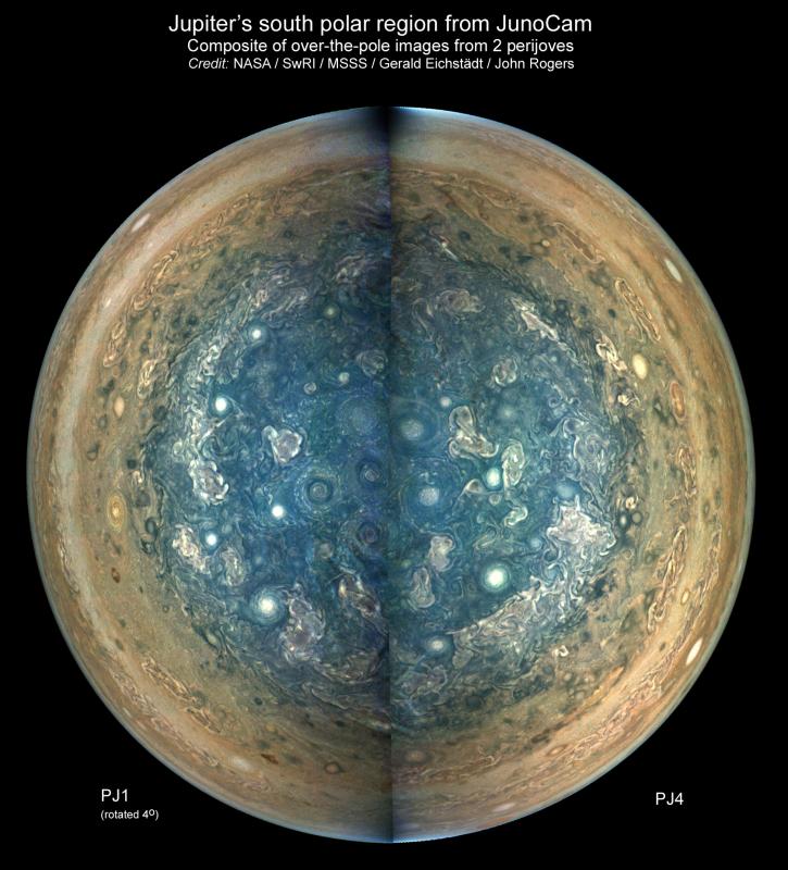
Figure 1.  South polar view of the planet, composited from views directly above the pole at perijoves 1 and 4.  In Figures 1-4, the component maps were correctly aligned in System III longitude (L3), except for rotations of a few degrees, and small offsets, to optimise the register of the CPCs.

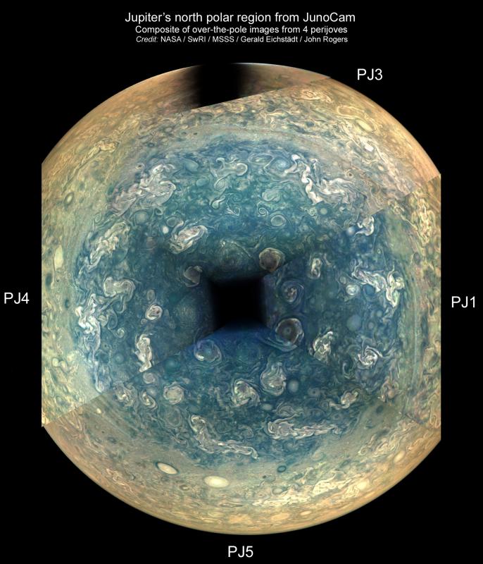
Figure 2.  North polar view of the planet, composited from views directly above the pole at perijoves 1, 3, 4 & 5.  (Small rotations and offsets were applied but are not indicated.)

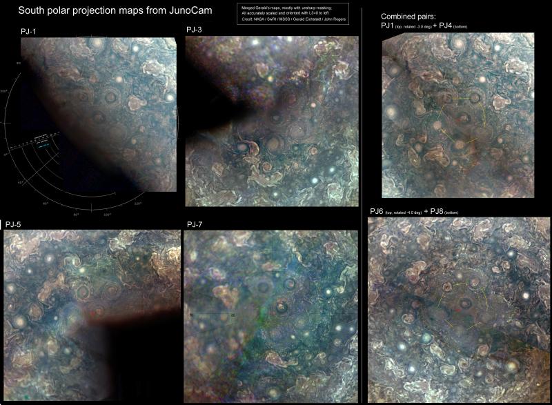
Figure 3.  South polar projection maps of the CPCs at single perijoves (PJ-1, 3, 5, & 7) and in pairs with the pentagon delineated (PJ-1&4, PJ-6&8).  Red crosses mark the south pole. 

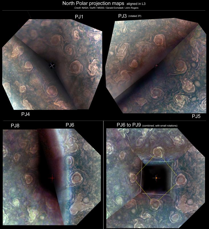
Figure 4.  North polar projection maps of the CPCs composited from pairs of perijoves (PJ1 to PJ6) and from four perijoves with the ditetragon delineated (PJ6 to PJ9).

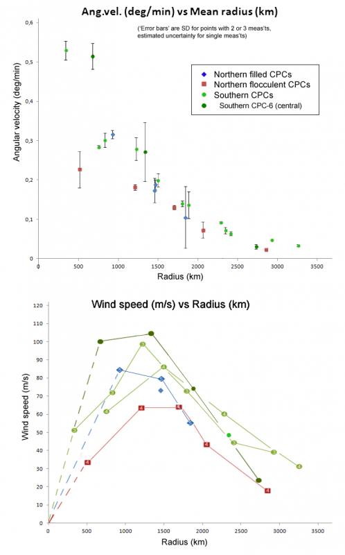
Figure 5.  Angular velocities and wind speeds within the CPCs at PJ3, measured by JHR from JunoCam images projected by GE. In the lower panel, individual CPCs are colour-coded and connected by lines.  (Similar results were obtained from images at PJ1 and PJ4, not shown here.)

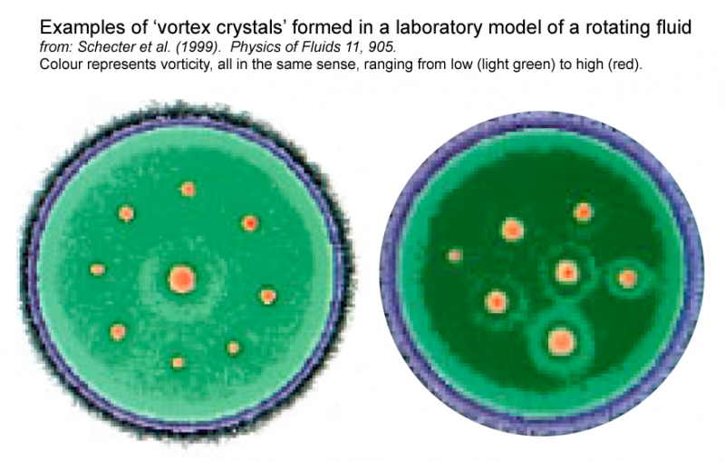
Figure 6:  Examples of ‘vortex crystals’ formed in magnetized electron columns, a laboratory model of non-viscous fluid turbulence, as shown in [ref.5]. (Colour represents vorticity, all in the same sense, ranging from low (light green) to high (red).)  

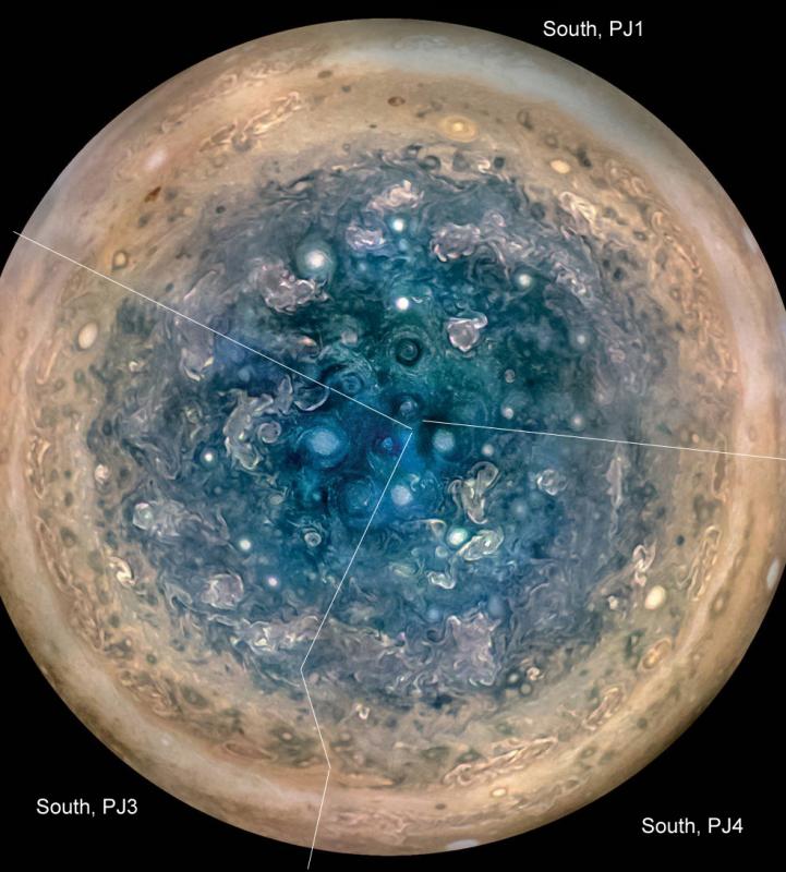
Figure 7.  This composite south polar view of the planet, released by NASA on 2017 May 25, was a compilation of views from 3 different perijoves, as indicated here.  As the pentagon of cyclones is not centred on the pole, it was not coherently shown in this compilation.  Original image credit: NASA/JPL-Caltech/SwRI/ MSSS/Betsy Asher Hall/Gervasio Robles.

______________________________________________________________________________________________