Image denoising in astrophotography – an approach using recent network denoising models

2023 August 10

Scott Sloka

Image denoising is an important consideration for improving the accuracy of acquired data. Given the morphological nature of astrophotography, with sparse star data overlaid on dim underlying background nebulae and galaxies, denoising is complicated to implement. New methods using convolutional neural networks and transformer networks show promise in general denoising applications. This paper explores the use of five recent denoising networks on astrophotography image data and demonstrates the feasibility as well as optimisations and pitfalls in the use of these networks. The paper confirms that image denoising in astrophotography using such networks is accurate and that a complete knowledge of ground truth might not be necessary for the accurate training of them.

Introduction

Astrophotography is the acquisition of astronomical image data, usually from ground-based systems. Image denoising is a computational technique aimed at restoring a clean image from a noisy image. This noise can be accumulated from multiple different sources.¹ In amateur astrophotography, there are a few dominant sources of noise, namely shot noise, readout noise of the sensor, and any aberrations introduced by postprocessing.

Shot noise is the random fluctuation of photons incident upon the sensor: photons arrive via the imaging system at the surface area of each pixel in the sensor array, and it is the statistical variation of photon emissions over time from all sources. This shot noise is proportional to the sum of all sources of light, including photons from the astronomical object and light pollution. Electrons may also be generated from heat in the camera and produce a thermal signature called dark current. This dark current is often reduced with cooling and calibrated out with dark-frame calibration. Unwanted sources of light such as sky glow from light pollution may also be reduced by calibration.

Essentially, the goal of image denoising is to recover a clean image, x, from a noisy observation, y, which may be modelled as:

y = x + v

where v is the noise in the image from all sources, x is the clean image, and y is the image that is measured (imaged). Denoising comprises the methods that try to remove v from y to give the best estimate of x.

The reasons for denoising in astrophotography are multiple. For some, the cosmetic/visual improvement is desirable. Others may use the denoised image to attempt to model the noise, v, to get a better understanding of the imaging system. Still others may wish to take the denoised image to use for other applications such as photometry, astrometry, pattern recognition, or object discovery.

Previous approaches required an understanding of the physical properties of the multiple noise generation mechanisms, and may not be easily generalised if image acquisition conditions are not constant.^2–4 Although it is difficult to model the combination of different noise processes in a single mathematical model, one major advantage of these methods is the fact that they are mathematically based upon knowledge of the underlying processes, even given the inherent complexities of modelling these processes.

Another approach to reducing noise trains a model without full knowledge of the noise process. This new approach, using so-called ‘deep neural networks’, addresses noise reduction in image acquisition processes using machine-learning techniques. This requires knowledge of both clean (called ground truth, which is an ideal representation of the image) and noisy images for comparison, in order to train the denoising network. A deep neural network will be trained to then take a noisy image and produce a cleaner image, ideally very close to the ground truth. These methods effectively take large data sets and through the training of clean and noisy image pairs, develop a model of denoising based on the training data set.

One inherent difficulty with this method is the presence of problems with generalising from the training data set to images with characteristics that are not similar to the set. This is due to the fact that not all noise generation conditions may be encapsulated within the training data, and therefore not all possible ground-truth image characteristics are presented to the network for training. Additionally, overtraining of the training data can lead to a phenomenon called overfitting, which can introduce artifacts in tested images. Therefore, for these deep learning methods, optimal selection of training images improves accuracy and generalisability.

These deep learning methods produce results that are an improvement on the noisy images used as input and are therefore ‘denoised’. A standard analytic/equation-based denoising algorithm, called BM3D, is used as a benchmark to determine if there is an improvement over this relative reference.

Convolutional neural networks (CNNs) are a type of deep learning method that, in some sense, model the properties of certain biological vision systems. These algorithms have multiple layers that may represent different features within the image. The structure of these network models affects the accuracy and generalisability of the outputs, as suggested above, and many such algorithms are optimised to address issues such as overfitting (does the algorithm introduce outputs only from its training set?) and generalisability (is the algorithm flexible enough to address data that it has never seen before?). Another novel and recently popular approach to image denoising is to use algorithm structures called transformers.⁵ Instead of using deep CNNs, this approach uses feature extraction at different resolutions to try to model the transformation of input to output.

Some of these algorithms are quite complex, requiring lengthy training times and lengthy denoising times, necessitating implementation on parallel processors such as graphical processing units (GPUs).^4,6 Therefore, high performance is sometimes traded off with respect to computational efficiency, with possibly lower accuracy of results. Also, some of these methods necessitate selecting manually chosen parameters in order to enhance the generalising performance.

CNNs have been demonstrated to be capable of image denoising using an unsupervised learning approach.⁷ CNNs are able to successfully remove Gaussian noise.⁸ Different network models have been successful and able to achieve performance comparable to BM3D,^9,10 but they need to be trained for a certain noise level, making these approaches less optimal because the noise level for any given image might not be known. Further models such as DnCNN,¹¹ VDNet,¹² and possibly FFDNet,¹³ have been successful at general image denoising for multiple noise levels and accounting for the spatial variance of noise across the image.

CNNs have several advantages over other denoising algorithms.¹¹ With very deep architectures – i.e., many layers – CNNs are effective at optimising denoising across variations in image characteristics.¹⁴ Also, implementation of these methods has been improved with optimised learning techniques.^15,16,17 These techniques improve the training process, thereby improving the denoising performance. One other major optimisation is that these methods are highly parallel and can successfully employ modern GPUs to exploit runtime performance.

Some CNN models have been successful at other aspects of image processing such as image super-resolution and JPEG image deblocking,¹¹ suggesting that some of these architectures may be generalisable to more than just image denoising. These implementations of CNNs have been shown to outperform state-of-the-art methods such as BM3D,¹⁸ WNNM,⁴ and TNRD.¹⁰

Methods

A series of simulated images was created to provide the means for a ground truth for comparison of methods, comprising several components. Stars were generated using PixInsight, version 1.8.8-12, with a script called CatalogStarGenerator, to generate several sets of stars with a point spread function based on the magnitude of the star. Stars were generated with their observed magnitude, and all stars within a region were generated with magnitudes of 17 or brighter using the VizierR star index. Generated images were 4096×4096 pixels; the star fields were generated with a pixel size of 9×9µm and a focal length of 530mm. This was to mimic the specifications of the imaging system discussed later. Star fields from the regions of M45, M81, the Fireworks Galaxy (NGC 6946), and the Iris Nebula (NGC 7023) were generated to get a variety of star configurations.

Nebula fields were simulated using Blender, version 3.1.0. A methodology of generating relatively smooth but finely detailed patterns was used. Galaxies were simulated by Gaussian bumps generated using Python code and warped using Photoshop. The stars, simulated nebulae, simulated galaxies and empty-space backgrounds were combined, and the various combinations were used as ground-truth images to optimise various characteristics of astrophotography targets such as dense/sparse star fields, and the presence/absence of deep-sky objects such as nebulae and galaxies.

To simulate acquired images, Gaussian white noise was added to the ground truth images to generate 20 noise images. To simulate stacked images, images were stacked using a Winsorized median stacking algorithm commonly used in amateur astrophotography. Stacks of two, three, up to 20 acquired images were created, and the 15 stacked images were used as the ‘clean’ image to simulate the type of data available to train from acquired images given the lack of a true ground truth. The 15 simulated acquired images were used as the ‘noise’ images for the first simulation. A separately generated set of 16 were used as test images to test the results of the trained networks. A second trained network was created with the usual 15 noise images, and also including the stacks of two, three, up to 14 image stacks. This approach simulated data that would be available to astrophotographers and was used to simulate lowering levels of noise used to train the network.

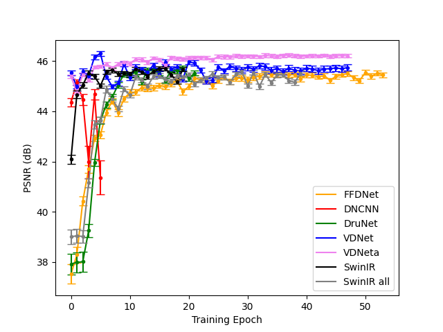
The training sets of images were used to train several models of CNN and transformer networks designed for image denoising. Implemented networks used in this analysis are listed in Table 1, and were modified according to the type of input used for the network.

(Log in to view the full illustrated article in PDF format)