Measuring the light profile of the Crab Nebula pulsar
2022 December 8
Historical round-up
In the year 1054, a new star appeared in the sky, close to the star known today as zeta Tauri. It was as bright as Jupiter, observable for many nights and visible even during the day. We know this because it was recorded by astrologers living in imperial China during the Song dynasty.
Winding the clock forward 700 years, an English amateur astronomer called John Bevis discovered a cloudy patch in the same region of Taurus whilst compiling a new atlas of the stars. This information was relayed to Charles Messier, who included it as the first entry (M1) in his famous catalogue of 1774. The same object was later observed in 1844 in Ireland by the third Earl of Rosse, using his self-built world-class telescopes. The high aperture of these telescopes enabled structure to be resolved within the nebulous object, which he subsequently named the Crab Nebula.
In the early 20th century, astronomers studied the nebula with increasingly large and more sophisticated instruments. Work carried out at the Lowell and Mt Wilson observatories in the US revealed that it was expanding and, by extrapolating backwards, showed that the nebula’s age was approximately 900 years. This important finding, along with other information such as location, led to the now accepted conclusion that the observation of 1054 and the Crab Nebula are connected. The event was in fact a supernova (SN 1054) that resulted in the nebulous remnant that we see today.
The discovery of pulsars & the physics of neutron stars
In 1967, Jocelyn Bell, a research student working on a radio telescope designed by Antony Hewish in Cambridge, England, detected a signal which pulsed every 1.3 seconds. Normally this type of repetitive signal was attributed to terrestrial noise and therefore dismissed. However, Bell and Hewish realised that it was coming from a fixed location in the sky (Vulpecula) and decided its origin must be extra-terrestrial. Bell went on to discover several similar signals and the Cambridge team realised then that they had discovered something new, predicting (correctly) that the signals were related to a compact star. It did not take long for the astronomical community to formally associate these signals with that of a hypothetical object known as a (spinning) neutron star, which was theorised back in the 1930s by Baade and Zwicky in the US. Once the first pulsing neutron star (now christened a ‘pulsar’) had been officially discovered, the subsequent astronomical ‘gold rush’ quickly resulted in more discoveries.
When a star of particular size (tens of solar masses) ends its life, the inward gravitational force of the outer material overcomes the dying thermonuclear outward pressure of the core. The star now has no option but to collapse in on itself and trigger a supernova. The outer layers are thrown off to form a nebula, whilst the inner layers continue to collapse. The ever-increasing pressure of the collapsing matter causes the constituent protons and electrons to combine to create neutrons, obeying the fundamental physical law of charge conservation. As the energy states of the atomic nuclei become filled, quantum mechanics dictates that any further collapse is no longer possible, and a neutron star is born.
The volume of an atom is normally defined by its outer electrons, meaning that an atom consists mostly of empty space. When these electrons combine with the protons, the atomic density rises sharply to equal that of the nucleus. This happens to the extent that the neutron star resulting from the collapsing matter has a radius of only tens of kilometres, containing up to several solar masses. As the dying star shrinks, its angular momentum is also conserved, resulting in a significant increase in rotation speed.
Even with all these extraordinary parameters, the star is now effectively dead and such an object would normally be undetectable. However, there is a way we can observe them. Like the parameters we have already discussed, the magnetic field, too, is scaled up. The immensely strong field accelerates charged particles up from the star’s surface. This produces a bipolar beam of radiation that emanates from the magnetic poles, which are normally offset from the spin axis. If this radiation sweeps across Earth, then we can detect the presence of the neutron star.
The Crab pulsar
In 1968, astronomers at the Arecibo Observatory in Puerto Rico observed a pulsar radio signal coming from the Crab Nebula. They made the astounding discovery that it was pulsing every 33 milliseconds, meaning that it was rotating about 30 times a second.
Up until now, pulsars were only associated with the emission of radio waves. But, like other objects we observe in the universe, they were thought to emit radiation across a broad range of the electromagnetic spectrum, including visible light.
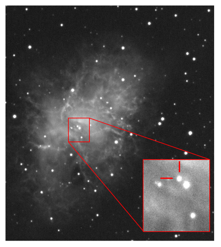
In 1969, a group of astronomers using a 36-inch telescope at the Steward Observatory in Arizona made the bold decision to try to detect a visible signal in the region of the Crab pulsar already identified by the radio signal. The exact location of the radio pulsar, designated PSR B0531+21, was still not known. Armed with an electronic light detector and a specialised piece of equipment called a Computer of Averaging Transients, their efforts were quickly rewarded by the detection of a star that was indeed flashing at the same rate as the radio signal. Figure 1 shows the location of this star.
Optical detection using amateur equipment
Pulsars are difficult objects for the amateur to observe. The main problems are firstly that they are faint, and secondly that they are usually flashing many times a second. If we are going to attempt to detect a signal and ideally construct a light curve (brightness vs. time) to identify a pulse profile, then it is best to do so in the optical band. This should be possible with any current-day moderate telescope, drive, and camera system. Optical pulsars are rare but as we have seen, PSR B0531+21 is a prime candidate for us, with an apparent magnitude of 16.5.
Our main problem is the exposure time required, which is dependent on factors like telescope aperture and camera sensitivity. At best, it will take a few seconds to obtain a suitable image. This will far exceed the pulse period that would have flashed hundreds of times during the exposure, making it impossible to detect any pulse. How does one take a series of images over the period of a single pulse, that will enable a representable light curve to be plotted?
One method available to us is to block the light source from entering the camera over the pulse period, except for a small repeating window. If the period of the window is less than the period of the pulse and synchronised, then it will be possible to detect a small region of the light curve. Admittedly we are now blocking out more light from entering the camera, so a longer exposure time will be required. However, this does not matter as the camera will always be looking at the same region of the repeating pulse, so we can integrate for as long as we like. Now, if the window frequency was to be set slightly out of phase with that of the pulsar, then the observed region would shift slowly across the window with respect to time. This means that we should now be able to obtain a set of consecutive images that represent the varying brightness of the pulsar. This ‘stroboscopic’ method, based on a mechanical light chopper, has been carried out successfully in the past. A paper by Kotar et al. (2003) describes one such example.1
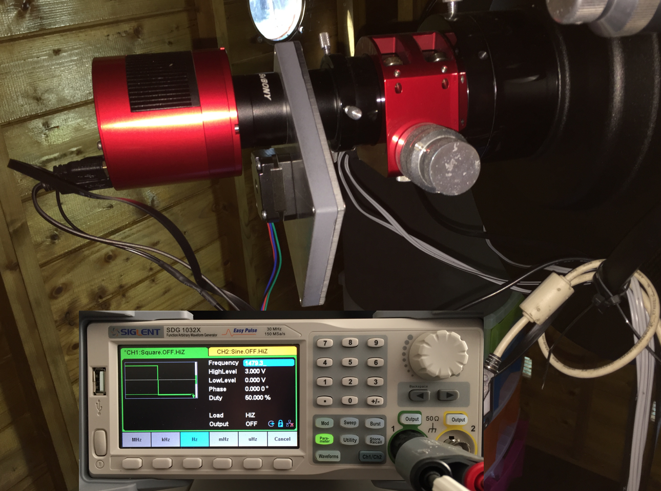
The remainder of this article discusses a system and process based on a similar device, along with the results obtained. The light-chopping unit used was of simple construction, consisting of a thin box containing a rotating metallic disc driven by a stepping DC motor. The disc had four segments cut out that allowed the light to pass through. These were placed at even intervals around the disc, providing four exposure windows per revolution as well as serving to keep the device balanced. This was particularly important as the disc needed to spin at a high rate. The whole unit sat between the telescope (14-inch Schmidt–Cassegrain) focuser and the camera (ASI 1600MM) – see Figure 2. A digital signal generator was used to drive the DC motor. Any stable selectable electronic square-wave source would suffice here, as long as it is capable of driving the motor/disc at an accurate rate.
A pulsar’s rate of spin slows down over time as a consequence of emitting radiation and PSR B0531+21 is actually spinning 0.5Hz slower than when it was discovered. The spin rate for the time of observation was obtained from the Jodrell Bank website, which gave it as 29.588Hz.2
The signal generator was configured to drive the disc so that a window would be presented over the camera at the equivalent frequency, which resulted in the disc rotating at 444rpm. The start-up/observation procedure was to first manually rotate the disc to place one of its windows over the camera. The pulsar was then located, auto-guiding started and focusing attempted. Note that a precise focus was not important, as photometric measurements were going to made on the images to find the sum of pixels in the region of interest. The signal generator was then started and repeat-imaging initiated, to find the ideal exposure time and rotation speed. This was so a reasonable number of samples could be collected to represent one or more pulses.
Depending on the initial settings, the monitoring could start anywhere within the pulse period. You will know immediately that the system is working when the star (pulsar) has disappeared or starts to fade away. For the system described here, a 20-second exposure (at maximum gain) was the minimum time required to capture a representative signal. The system was driven at a frequency to obtain approximately 100 images, covering one pulsar rotation period. It was found that fine adjustments of the signal generator frequency enabled this value to be reduced or increased as desired.
Processing the data
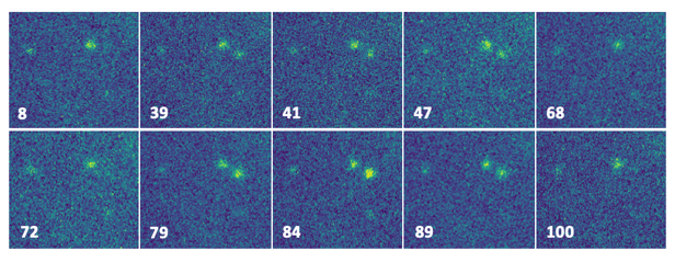
The data presented here were collected from an observation consisting of 200 images, using the procedure described above. All image and data processing was carried out using the Python scripting language and applicable libraries. The images were first dark-frame adjusted and then registered (aligned). Figure 3 shows a selection of the frames after the initial processing.
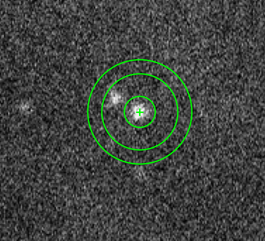
Aperture photometry was used to measure the brightness of the pulsar with respect to the background. The background mean value was calculated using an annulus aperture, carefully placed so as to miss other stars in the region (Figure 4).
Final results & thoughts
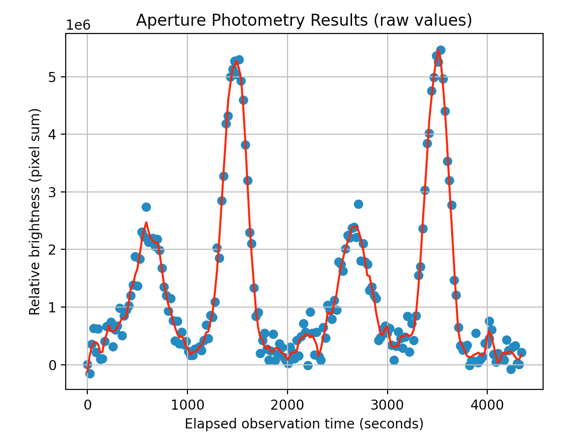
The result of the photometric analysis is shown in Figure 5. Each point on this plot shows the pulsar brightness (pixel sum) after background subtraction for a single 20-second exposure. It should be noted here that each rotation consists of a weaker interpulse as well as a main pulse.
As two complete rotations of data had been collected (more would have been better), it made sense to find the average profile, filtering out some of the noise. This was achieved by first determining the time for a single observed rotation and then folding the data so they laid over each other. Finally, binning was used to determine the mean values. The result (Figure 6) is a profile detailing one complete 360° revolution of the pulsar.
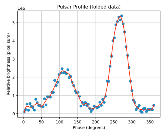
What does this profile show us? As already mentioned, it consists of two separate pulses. The accepted interpretation is that the neutron star’s magnetic dipole is perpendicular to its rotation axis, and Earth is lying on its equatorial plane.3 The plot shows the separation between the pulses to be approximately 180°, which further supports this explanation. The variation of width and brightness between the pulses indicates that we are observing different regions and intensities of the beamed radiation cones.
It should be noted that the stroboscopic method used here acquired the data over some 120,000 actual pulse periods. Thus, the profile obtained is very much an average representation. Also, the sliding window used for each exposure would have acted as a filter, removing any sharpness from the signal. However, even with these caveats, if we compare the profile with the many online publications, we see that it is highly representative of professional acquisitions in both shape and feature timings.
References
1 Kotar J., Vidrih S. & Čadež A., ‘Charge coupled device based phase resolved stroboscopic photometry of pulsars’, Review of Scientific Instruments, vol. 74 (2003): 10.1063/1.1571949
2 jb.man.ac.uk/~pulsar/crab.html (accessed 2022 October)
3 Lyne A. & Graham-Smith F., Pulsar Astronomy, Cambridge University Press, 1998
| The British Astronomical Association supports amateur astronomers around the UK and the rest of the world. Find out more about the BAA or join us. |