Observing exoplanets with the MicroObservatory: 43 new transit light curves of the hot Jupiter HAT-P-32b

2021 November 30

Martin J. F. Fowler, Frank F. Sienkiewicz, Robert T. Zellem & Mary E. Dussault

Introduction

Over two decades on from the discovery of the first planet orbiting a main-sequence star other than our own Sun,¹ the number of confirmed exoplanets in the NASA Exoplanet Archive as of 2020 May 21 was 4,158, with a similar number of candidates awaiting confirmation.^2,3 The diversity of such worlds spans a much wider range of physical conditions than those in our solar system and form a continuum, from gas giants composed mostly of hydrogen, to smaller ocean planets where water may provide most of the mass, to rock-iron terrestrial worlds in some ways similar to the Earth.⁴ One particular group of exoplanets with no solar-system counterpart is known as the ‘hot Jupiters’ class. These planets have masses comparable to, or greater than, Jupiter but orbit very close to their primary star (i.e., within 0.1au). Exoplanets appear to be ubiquitous and it is estimated that for the stars that have been searched most thoroughly, i.e., main-sequence dwarfs of 0.5–1.0 solar masses (M_☉), the probability that a random star has a planet is of the order of unity.⁵

Under the fortuitous condition that the orbital plane of a planetary system is coincident with the observer’s line of sight, exoplanets can be observed to transit their host star, leading to a periodic slight dimming of the star.⁶ Known as the ‘transit method’, this technique has been used to great effect by ground-based observatories such as the Hungarian-made Automated Telescope Network (HATNet),⁷ and the Wide Angle Search for Planets (WASP),⁸ as well as the space-based missions CoRoT, Kepler and, currently, the Transiting Exoplanet Survey Satellite (TESS).⁹ To date, Kepler has been responsible for the discovery of most of the known exoplanets,¹⁰ and TESS is predicted to discover >10,000 new transiting examples.¹¹

Relatively modest equipment, such as a 0.25m Schmidt–Cassegrain telescope on an equatorial mount, can be used by amateur astronomers to yield high-precision transit light curves of hot-Jupiter exoplanets.¹² The Exoplanet Transit Database (ETD), run by the Czech Astronomical Society,¹³ currently includes data on >9,500 transits of over 350 exoplanets, the majority contributed by amateur observers. Amateur data from the ETD and other sources have been used to investigate transit timing variations,^14,15 as well as for the refinement of ephemerides of transiting exoplanets with high timing uncertainties.¹⁶

Indeed, observations of transiting exoplanets by amateurs and other users of small telescopes (≤1m), have an important role to play in the maintenance of the ephemerides of targets for future space-based telescope missions.^17,18 These missions include the NASA James Webb Space Telescope (JWST, 2021 launch), the ESA ARIEL mission (2028 launch), and an Astro2020 Decadal mission (~2030 launch). Without follow-up by ground-based observations, the ephemerides of many of these targets would become ‘stale’ by the time the missions are flown, leading to the prospect of inefficient use of valuable telescope time because of the uncertainty in the transit timings. To this end, projects such as NASA Exoplanet Watch and ARIEL ExoClock,^17,19,20,21 both of which are open to amateur observers and other users of small telescopes, have been established to monitor transiting exoplanets in order to keep their ephemerides up to date.

Observations of transiting exoplanets also form the basis of the Laboratory for the Study of Exoplanets (ExoLab), an online teaching resource that is operated by the Science Education Department at the Center for Astrophysics, Harvard & Smithsonian.^22,23 Developed with funding from the US National Science Foundation, and aimed at high-school classrooms in physics, astronomy and Earth science, ExoLab uses the 6-inch (152mm) telescopes of the MicroObservatory robotic telescope network to enable students to detect and analyse the transits of known exoplanets using rudimentary online photometry and modelling tools. Since 2009, MicroObservatory has taken >3,500 transit datasets to serve science students and interested exoplanet observers.

Complementing ExoLab, the ‘DIY Planet Search’ website – a project of NASA’s Universe of Learning^24,25 – is a public engagement tool that uses the same image data as ExoLab and allows anyone to investigate the transit method. Whilst a similar online photometry tool is provided on the website, the images can be downloaded as FITS files for offline reduction and analysis.²⁶ Importantly, these are all new observations; over the course of a year many are made of around 30 known exoplanets.

One of the targets regularly observed by DIY Planet Search is the V = 11.3mag, late-F–early-G dwarf star GSC 3281-00800 (= HAT-P-32), which is orbited by the exoplanet HAT-P-32b. Discovered by the HATNet in 2004 and confirmed some seven years later, HAT-P-32b was initially found to have a mass of ~0.86M_J, radius of ~1.789R_J, transit depth of the order of 20 millimagnitudes and an orbital period, P, of ~2.15d.²⁷ The mass and radius estimates were subsequently refined to 0.68M_J and 1.98R_J respectively.²⁸ The planet’s dayside temperature has been measured by Zhao et al. (2014) to be T_eq = 2,042 ± 50K,²⁹ and its optical transmission spectrum shows little variation, suggesting a high-altitude cloud layer masking any atmospheric features.^30–33 Seeliger et al. (2014) have shown from transit timing analysis that the HAT-P-32 system does not exhibit transit timing variations (TTVs), arising from additional unknown bodies, of more than ~1.5min,³⁴ making it a good target to evaluate the accuracy and suitability of MicroObservatory observations for exoplanet research.

In this paper, we present observations of 43 transits of exoplanet HAT-P-32b by the MicroObservatory together with estimates of the parameters of the system based on the analysis of combined transit light curves, and an updated ephemeris.

Observations

Between 2013 and 2020, 43 complete transits by HAT-P-32b were successfully observed by the MicroObservatory robotic telescopes (Table 1). During this period, observations of a further 40 transit events were attempted, of which 11 provided partial transits and the remainder were unsuccessful either because of: technical issues (10); poor weather (14); or very noisy transits that could not be analysed successfully (5). Overall, the success rate of observing complete HAT-P-32b transits was ~52%.

Except for the observations of 2014 Oct 4, which were made using the MicroObservatory telescope Donald, all the observations were made with the telescope Cecilia.³⁵ Located at the Smithsonian’s Fred Lawrence Whipple Observatory (FLWO) in Amado, Arizona, USA, the MicroObservatory telescopes are of an original Maksutov design, with a 6-inch [152mm] spherical primary mirror and a focal length of 560mm.²² A Kodak KAF-1402ME CCD sensor produces images covering a field of view of 0.96×0.75°, with a nominal plate scale of 5.21 arcsec/pixel (2×2 binning). For each observation run, we obtained unfiltered 60s-exposure science FITS images with a three-minute cadence, from around one hour before and one hour after the predicted start/end of the transit, giving approximately 100 images per run. The headers of the FITS images were time-stamped with the start of exposure based on a local precise time server at the FLWO and are accurate to the nearest second.

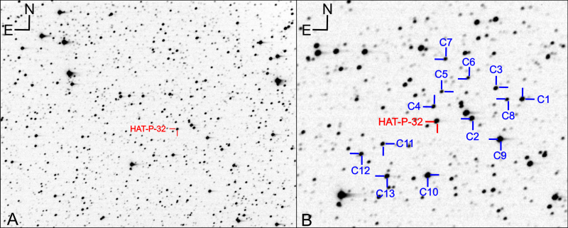
In addition to the science images, two dark-field images were collected on each run. Whilst flat-field (FF) images were not available, for the 2016 runs which were particularly noisy with dust motes, a master pseudo-FF was prepared from nine images of the exoplanetary system WASP-52, obtained on an overcast moonlit night. This pseudo-FF to some extent offset the ‘wandering’ of the target and comparison stars across the sensor throughout the sequence of images, although this remains a significant source of noise in the datasets. A representative science image showing the HAT-P-32 field is shown in Figure 1.

Data reduction & analysis pipeline

We developed a partially automated MicroObservatory Exoplanet Observation Workflow pipeline (MEOW v. 1.0) for the reduction and analysis of the DIY Planet Search images. For each set of observations, the science images, together with a dark-field image and, where available, the pseudo-FF image were imported into MuniWin (v. 2.1.24 (×64)),³⁶ for automated differential aperture photometry using an ensemble of up to eight comparison stars as shown in Figure 1 and detailed in Table 1. The measuring aperture was typically three pixels in radius and the background sky was measured using a concentric aperture of two pixels, with a gap of one pixel between the two apertures. We then saved the photometry output from MuniWin (Julian Date (JD_UTC) of mid-observation, V–C magnitude, error), together with the airmass, as text files and uploaded the photometry output to the ETD to gain an initial indication of the quality of the transit (Level 1 analysis).

For more detailed analysis, we imported the text file outputs from MuniWin into a custom Microsoft Excel spreadsheet for conversion into a format suitable for use with the EXOFAST transit-fitting model developed by Eastman et al. (2013).³⁷ For this higher-fidelity analysis (Level 2), the V–C magnitudes were converted to relative fluxes and the time converted from JD_UTC to Barycentric Julian Date in Barycentric Dynamical Time (BJD_TDB) using the online utility developed by Eastman et al. (2010).³⁸ For each data point, a linear de-trend parameter was calculated based on the slope of the pre- and post-transit data points as identified from the Level 1 analysis, and the fluxes normalised to an out-of-transit value of ~1. We then prepared an ‘output’ text file comprising: BJD_TDB, normalised flux, flux error, linear de-trend parameter and airmass. This file was used as the photometry input to the EXOFAST transit-fitting model.

A full demonstration of the use of MuniWin software with MicroObservatory exoplanet image data is available on YouTube.³⁹

Transit-fitting modelling

EXOFAST has become an important tool for astronomers who want to use transit light curves or radial velocity data, or both, together with various inputs, to create models of planetary systems. Originally requiring the use of the proprietary software language IDL, the NASA Exoplanet Archive has recently integrated the same IDL-based calculations as the original into its suite of web resources.³ The software implements the light curve models of Mandel & Agol (2002),⁴⁰ as well as a differential-evolution Markov Chain Monte Carlo (MCMC) method,^41,42 to estimate and characterise parameters and uncertainty distributions.⁴³ The Exoplanet Archive website provides enough back-end computing resources to enable the MCMC analysis of observed transit light curves and thus relieves the user of the need to run this high-fidelity model locally.

We uploaded individual output photometry files from the MEOW pipeline to EXOFAST, and the default parameter set for HAT-P-32b required for the model was ‘pulled’ from the Exoplanet Archive. The various prior values of the required parameters, hereafter termed ‘priors’, together with their widths (uncertainties) are given in Table 2. These priors represent the default parameter values for the system in late 2016 and whilst they have been updated since then, these have been used in the analysis to maintain continuity across the observation datasets. Limb-darkening coefficients were automatically calculated by EXOFAST for each run. Except for the run using combined transits covering multiple epochs, a mid-transit (T_C) prior was not specified since for transit-only fits the mean of the input times is used by the model as the prior when no midpoint is specified.

With transit-only fits, the light-curve data alone provide very little constraint on the eccentricity and longitude of periastron, both of which are required for the model. These parameters appreciably affect the derived physical parameters. Accordingly, we forced a circular orbit for the transit fits, as recommended by the EXOFAST documentation. Such an orbit is consistent with the near-circular solution of Zhao et al. (2014),²⁹ although others have derived eccentricities in the range 0.10–0.22.^27,28

(Login or click above to view the full illustrated article in PDF format)