Saturn during the 2005/2006 apparition

2020 March 30

Mike Foulkes

Introduction

This apparition commenced after solar conjunction on 2005 Jul 23.¹ Opposition was on 2006 Jan 27,² when the planet was in the constellation of Cancer and lying at the southern edge of the Beehive Cluster. At opposition, the planet’s apparent magnitude was –0.2; its apparent equatorial diameter was 20.4″ and the apparent major axis of the rings was 46.2″. This apparition finished at solar conjunction on 2006 Aug 7.²

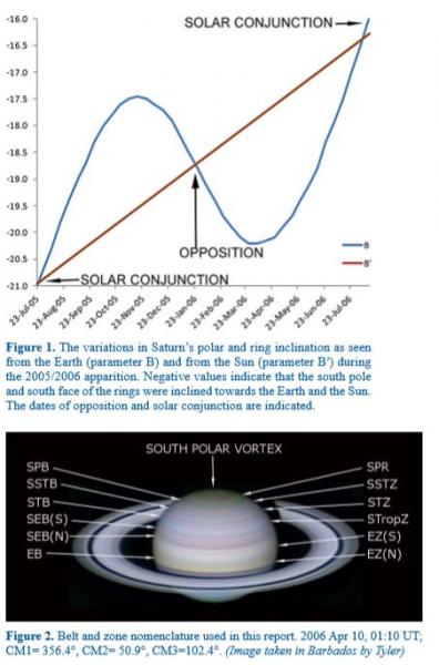The variation of the apparent inclination of its pole and rings with respect to both the Earth and the Sun during this apparition is shown in Figure 1.

At opposition the ring inclination with respect to the Earth was –18.9°.

Observations

A large number of observers contributed to this report, with the majority using digital imaging techniques. Those who contributed visual observations are shown in Table 1. Table 2 shows those who provided digital images.

The first observation of this apparition was made on 2005 Sept 23 by Maxson and the last was made by McKim on 2006 May 30. The largest telescopes used were by Gray, McKim and Parker, with apertures of over 400mm. Some images were taken with colour cameras, but a number of observers used red, green and blue filters to construct colour images. Some observers also used infrared (IR) and ultraviolet (UV) filters, as shown in Table 2.

During 2006 April, Kingsley, Peach and Tyler made an expedition to Barbados to image the planets under favourable seeing.³ Their observation programme concentrated on Jupiter and Mars, but a number of Saturn images were also taken. Peach was able to provide images from Apr 8–23 inclusive.

The WinJUPOS software was used to derive spot longitudes, ⁴ average spot drifts and belt latitudes.

Nomenclature & terminology

Abbreviations and terminology are as defined in ref. 5. All drawings and images shown in this report are orientated with south upwards and with the preceding (p.) edge to the left. Planetographic latitudes (the default in WinJUPOS) are used unless otherwise stated.

Figure 2 shows the belt and zone nomenclature used in this report.

Latitudes

Latitudes of the edges of the belts were derived by measuring a number of the best colour images using the WinJUPOS software. Table 3 shows the derived latitudes; values are given in both the planetographic and planetocentric systems.

The standard deviations given in Table 3 were derived from the individual measurements. However, it is likely that the uncertainty of the latitudes may be higher than this.

No significant changes in belt latitudes were observed during this apparition. The latitude estimates show that the Equatorial Belt (EB) was asymmetrically placed with respect to the planet’s equator, i.e. it lay predominantly in the southern hemisphere. The bright bluish-coloured zone in the northern hemisphere has been designated as the North Temperate Zone (NTZ) for the purposes of this report, although its true designation is uncertain.

The derived latitudes of the southern hemisphere belts are comparable with those found during the previous apparition.⁶ However a full comparison of the southern hemisphere belt latitudes over apparitions recent, earlier and subsequent to this one will be given in a later apparition report.

Visual intensity & colour observations

Only four observers provided visual intensity estimates of the belts and zones; these are shown in Table 4. Gray made the largest number of estimates. No colour filters were used in these observations. For each belt or zone, the table gives the average value derived by each observer plus the overall average based on all observations.

There are differences in the values recorded by some observers for certain features. However the results show the EZ(S) to be the brightest zone and the SEB(N) & SPB to be the darkest belts.

Visual colour estimates of the belts and zones are shown in Table 5. This table also shows a visual assessment by the author of the colours shown in the colour images.

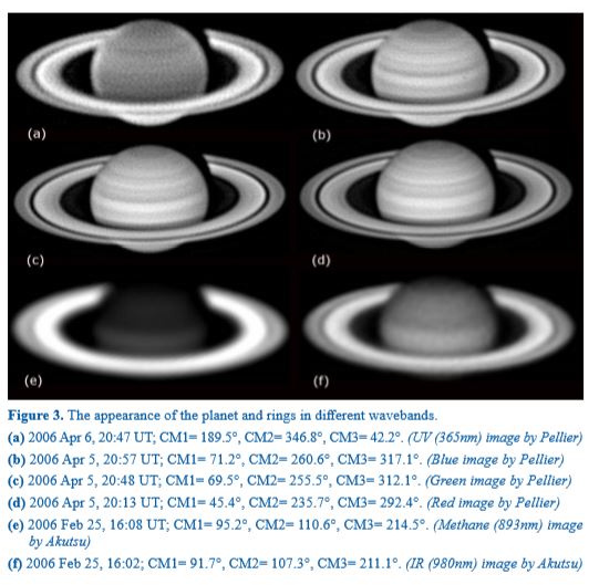
During this apparition, a number of images were taken using a variety of filters ranging from UV up to the near-IR. Typical examples of these observations are shown in Figure 3, although these images were taken by different observers using a variety of equipment and on different dates.

In UV (365nm), some regions of the planet appeared light, although the South Polar Region (SPR) and South Temperate Belt (STB) appeared dark (Figure 3a). The EZ also appeared dark.

Methane is a constituent of Saturn’s atmosphere and this molecule very strongly absorbs light at 890nm. Light is reflected from high-altitude clouds in the upper atmosphere with less methane light absorption at this wavelength than lower-level clouds. Consequently, higher clouds appear bright and lower clouds dark in images taken with methane filters. During the apparition much of the planet appeared dark at this wavelength, although the EZ appeared light, therefore indicating relative height (Figure 3e). The STropZ also appeared light, but not as bright as the EZ.

Rings A & B were visible with all the filters used in Figure 3.

(Login or click above to view the full illustrated article in PDF format)