Saturn during the 2009/2010 apparition
2023 February 7
A report of the Saturn Section. Director: Mike Foulkes
This report describes observations of Saturn made during the 2009/2010 apparition. The evolution of a storm system that appeared in the South Tropical Zone is discussed, as well as observations of a long-lived white spot that was in the South Equatorial Belt Zone. Also presented is the appearance of the belts and zones; especially that of the North Equatorial Belt (NEB). At low resolution, the NEB often appeared as a single diffuse band. The NEB(N) was darker than the NEB(S) and the southern component of the NEB(N) was often the darkest. Observations of some satellite phenomena are also presented.
Introduction
This apparition commenced at the solar conjunction on 2009 Sep 17,1 and finished at the solar conjunction on 2010 Oct 1.2
Opposition was on 2010 Mar 22,2 with the planet in the constellation of Virgo. It lay just north of the celestial equator, with a declination of just under two degrees. At this time, the planet’s magnitude was 0.5, with an equatorial diameter of 19.5ʺ and the major axis of the rings at 44.7ʺ.
The Sun and Earth passed through the ring plane on 2009 Aug 11 and Sep 4 respectively, after which the north face of the rings was presented to both the Sun and Earth.
The variation of the inclination of the pole and rings to Earth during this apparition can be found in the BAA Handbooks for 2009 and 2010,1,2 or by using the WinJUPOS software.3 The latter also allows the inclinations of the pole and rings to the Sun to be derived. The north pole and rings reached a maximum inclination of 4.9° during early January, and a minimum inclination of ~1.7° at the end of May. At opposition, their inclination was 3.1°. The inclination to the Sun and Earth became identical a few days before opposition.
Observations
Table 1 shows the observers who contributed observations for this apparition. A wide variety of instrumentation was used to observe the planet during this apparition. The majority of observations were made by digital imaging.
The first observation for this apparition was made by Sussenbach on 2009 Oct 6 and the last was made by Colombo on 2010 Aug 7.
Nomenclature & terminology
The belts and zones nomenclature used in this paper is that used in the previous apparition report.4 Some observers used slightly different nomenclature. For example, the northern component of the South Equatorial Belt (SEB(N)) was sometimes described as the SEB by certain observers, although the measured latitudes matched that of the SEB(N) in recent apparition reports. In such cases, the belt and zone designations were adjusted to match those given in this report.
Terminology is as per Foulkes (2010).5 All drawings and images are orientated with south at the top. All latitudes are planetographic unless otherwise stated.
Latitudes
Belt latitudes (Table 2) were derived from the belt colour images using WinJUPOS.3
A number of the belts appeared diffuse, as noted below. Consequently, in some cases, the measurement of belt latitudes was more difficult. Given this, the uncertainty in the derived belt latitudes is likely higher than the measurement standard deviations shown in Table 2.
The latitudes derived for the belt edges during this apparition are comparable with those obtained during the previous apparition,4 allowing for measurement error.
Visual intensity & colour observations
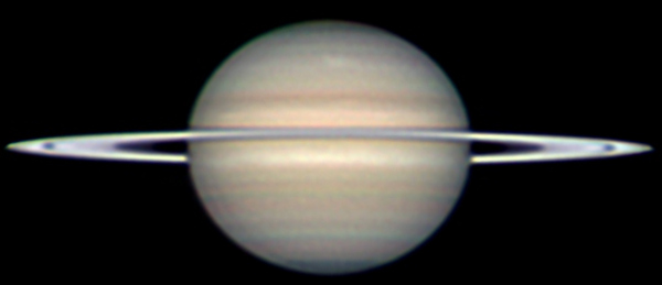
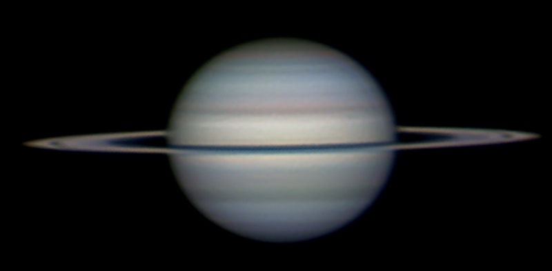
A comparison in the belt and zone structure for this apparition compared to that of the previous apparition can be made by comparing Figures 1 & 2. Figure 2 has been taken from Figure 2 of Foulkes (2013).4
One of the most striking features of this apparition was the appearance of the belts and zones, particularly the NEB which often appeared diffuse. This is shown in the images contained in this report. Some visual observations of the belt structure are shown in Figure 3. Visually, Heath noted the weakness in intensity of the belts on Mar 6.
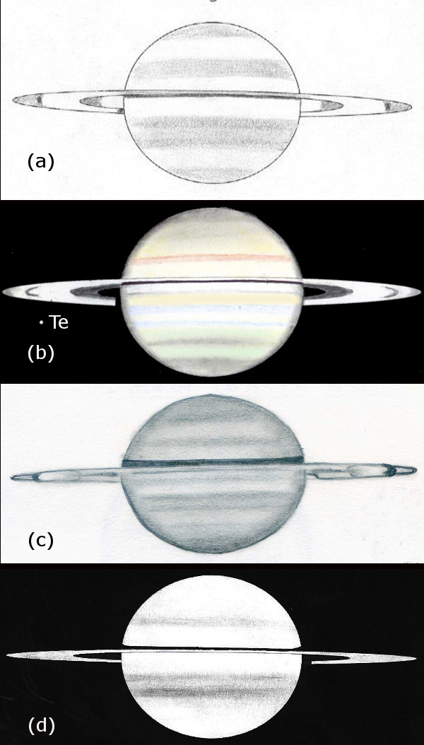
(a) 2010 Feb 13, 23:15 UT; CM1= 43.9°, CM2 = 47.0°, CM3 = 202.8°. (Drawing by Adamoli; 235mm SCT.)
(b) 2010 Mar 2, 00:46 UT; CM1 = 284.0°, CM2 = 128.4°, CM3 = 264.9°. (Drawing by Abel; 203mm Newt.) This drawing shows Tethys (labelled as ‘Te’) Np. of the planet.
(c) 2010 May 12, 20:30 UT; CM1 = 86.1°, CM2 = 130.7°, CM3 = 180.6°. (Drawing by Graham; 150mm OG.)
(d) 2010 May 27, 20:45 UT; CM1 = 158.6°, CM2 = 78.4°, CM3 = 110.2°. (Drawing by Giuntoli; 203mm SCT.)
The most obvious belt was the SEB(N), with its noticeable red colouration. The SEB(S) was fainter than the SEB(N), and indeed fainter than the STB.
In contrast, the NEB was often difficult to distinguish from the remainder of the northern hemisphere, particularly at low and medium resolution. The fading of the NEB may have started during the latter part of the previous apparition.4
Higher-resolution observations resolved some components in the NEB. McKim noted the faintness of the NEB, with the northern component darker than the southern, but recorded them to be closer in intensity later in the apparition. He also noted the SEB(N) to be fainter than the NEB on Mar 5. However, Gray’s intensity observations (Table 3) showed the NEB(N) to be darker than the NEB(S). Further, some higher-resolution images sometimes showed the individual components of the NEB to be darker than the SEB(N). When resolved, the NTB appeared to be close to the intensity of the NEB.
Table 4 shows the visual colour estimates of the belts and zones, although only a limited number of such estimates were made. This table also gives the colour estimates by the author from the colour images received. There are some differences in the colours shown in images by different observers. This may be due to the aperture, camera, filters and processing used.
Despite these differences, some consistent colours were recorded, such as for the SEB(N). Generally, all observations show this to have had a red colouration. The highest-resolution images show the NTZ to have had a distinct blue or turquoise colour and the NNTZ to have had an orange or reddish colour (see for example Figure 1). On some images, this reddish colour seems to extend into the NNNTZ. Such a colour has been recorded at similar latitudes of the southern hemisphere during previous apparitions. (See for example Foulkes (2013).4)
The colour estimates of the NEB, its components and intermediate zones were however more diverse and ranged from cold through to warm colouration. For example, the individual NEB components shown in Figure 1 appeared a warm grey tone. In Figure 6(d), the belt appears red. In Figure 7(b), the individual components appear grey but with an overall green background. In Figure 8(c), the belt components appear warmer in tone. Lower-resolution visual observations recorded a grey colouration but McKim, using a large-aperture instrument, consistently recorded a reddish hue.
The reason for these variations in colour estimates is not clear and no obvious correlation of colour was found with date or longitude.
As in previous apparitions, a few observers imaged the planet using filters, with wavelengths ranging from the near ultraviolet (UV) up to the methane band (890nm). Some typical examples are shown in Figure 4.
In UV (Figure 4(a)), the rings appeared darker than at other wavelengths. Little was seen on the planet’s disc at this wavelength, although the equatorial regions were dark.
The SEB(N) appeared slightly darker in the blue and green images (Figures 4(b) & 4(c), respectively) compared to the red image (Figure 4(d)), thus indicating the red colouration described above.
The NEB structure was more obvious at longer wavelengths, particularly in infrared (IR), compared to the appearance in the blue image, as did some other belts (Figure 4(e)).
As in previous apparitions, the equatorial regions appeared bright and the remainder of the planet dark in the methane band (Figure 4(f)). This indicates relative height of the equatorial regions.
The planet
South Polar Region (SPR)
The south pole was slightly tilted away from Earth. No detail was observed in this region, which appeared dark grey although Gray frequently reported a South Polar Cap (SPC). The northern edge of the SPR was marked by a dark belt whose latitude (Table 2) is consistent with the South Polar Band (SPB) observed in earlier apparitions.
South South Temperate Belt (SSTB) & South South Temperate Zone (SSTZ)
A narrow and light SSTZ was sometimes observed south of the SSTB. The SSTB appeared as a narrow belt.
South Temperate Belt (STB) & South Temperate Zone (STZ)
The STZ was light and narrow.
The STB was a dark belt. High-resolution observations showed this to be double, with the southern component the darker.
South Tropical Zone (STropZ)
A major feature of the apparition was the bright storm system that appeared in this zone. This comprised one or more light or bright spots, which sometimes extended slightly into the northern edge of the STB.
One characteristic of a few of these spots was a rapid increase in brightness, followed by an expansion in longitude and then a fading. Another was the generation of a disturbed sector of the STropZ, which by Jun 3 extended just over 35° in longitude.
Figure 5 shows the measured System III longitudes, against time, of the centres of all light spots observed in this storm system. The solid lines shown in Figure 5 do not indicate the drifts of the individual spots, but rather link the centres of what are believed to be the same spots based on both the positional measurements and a review of all images. Some different interpretations of these data are possible, as there are some gaps in the coverage and some rapid changes were observed with timescales of a day.
The appearance of this storm is shown in Figures 1, 6, 7, & 8. As well as being recorded in colour images, it was also recorded in red light and in IR on Mar 13 (Figure 5(e)). Throughout this apparition, it was only recorded in images, apart from two visual observations made by Abel on Mar 15 & 23. Table 5 gives the derived average drifts, latitudes and sizes for some of the spots observed in this storm system. The first observation was made on Mar 6 by Akutsu (Figure 6(a)), when it appeared as a small light spot at System III longitude 1.6°. This is designated as no.1 in Figure 5.
A faint object at a similar longitude was only suspected in an image taken by Maxson two days earlier on Mar 4. Nothing obvious was detected in this longitude region in observations made prior to that date, i.e., by Wesley on Feb 26 and Mar 2.
Positional measurements of this spot from images taken during the first few days after its appearance indicate a small negative drift with respect to System III (Figure 5). However, this is uncertain given the limited time period of these measurements. After this time, a positive drift relative to System III was observed.
Over the next few days, the spot became brighter. It then began to expand in longitude, becoming more elliptical in shape but also beginning to fade (Figure 6(b)–(c)). This expansion may have been in the f. (following) direction, as the longitude of the centre of the spot seemed to move rapidly to f. in a few days; this is shown in Figure 5.
From Mar 18 (Figures 1 and 6(d) & (e)), higher-resolution observations showed it having a double structure. For the purposes of this report, the spot f. is designated no. 1A in Figure 5. Lower-resolution observations only revealed a single elongated object. If differing observations on the same night showed it both as single and double, only the observations that showed it to be double are shown in Figure 6 for clarity. However, all observations have been used in the overall analysis.
On Mar 22, the zone immediately f. these two spots appeared disturbed (Figure 1).
The storm was still visible on Mar 26, but Go’s colour image taken on Mar 30 (Figure 6(f)) showed no feature at this System III longitude, although a brighter STropZ was suspected in the blue image taken almost at the same time. Nor was anything visible there in another image taken by Go on Apr 3.
However, on Apr 7, a bright spot was again observed in this longitude region (Figure 7(a)). This is designated no. 2 in Figure 5. In a similar manner to spot no. 1, this too began to brighten and expand in size, and began to appear more elliptical (Figures 7(b) & (c)).
By Apr 16 (Figure 7(d)), parts of the STropZ some 18° f. no. 2 had become slightly lighter. On Apr 17, McKim recorded the zone to be brighter (CM3 = 74–88°). Furthermore, on Apr 19 a small bright area had formed Sp. of no. 2. This too brightened and over the next few days appeared brighter than no. 2 (Figure 7(e)), but subsequently they appeared of similar intensity and were in close contact on Apr 28 (Figure 7(f)). By May 1, both spots were only very faintly visible (Figure 8(a)).
On May 5, another spot had become bright. As its longitude lay on the extrapolated track of no. 2, this was assumed to be the latter undergoing another brightening; this is discussed further below. By May 9 & 10 (Figure 8(b) & (c)), this too had expanded, with the STropZ becoming more disturbed p. (Figure 8(d) & (e)).
By Jun 3, one small light spot was visible p. with two major bright spots further p. (Figure 8(f)), and as noted above, the storm system extended just over 35° in longitude.
Some other brighter areas were recorded in the STropZ by McKim on Mar 27 (CM3 = 309–314°) and on Apr 26 (CM3 = 174–185°).
Radio signatures associated with bright storms at this latitude have been detected by the Cassini spacecraft in orbit around Saturn. These have been shown to be caused by lightning activity, indicating that these storms are giant thunderstorms. The storm system observed during this apparition was also shown to be correlated with lightning activity.6 The detection of this lightning started on Feb 7 (designated as storm I in Fischer (2011),6 but no storms were detected in the Section observations until Mar 6. The lightning was detected until Jul 14 but no Section observations recorded a storm after Jun 3.
Table 5 shows that the drifts derived for these spots did differ considerably. Spots no. 1, 1A and especially 2A were observed over relatively short timescales and so their drifts may be considered to be more uncertain. Figure 5 indicates that spot no. 1 may initially have had a small negative drift with respect to System III during its first days of existence, before assuming a more positive drift. However, Table 5 only gives the overall average drift for this spot. There were no observations of spot no. 2 at the end of May and so its track extending into June, shown in Figure 5, is also more uncertain.
It is possible that spots no. 1 and no. 2 may be the same object. Certainly, the later part of the track of spot no. 1 shown in Figure 5 extrapolates close to the initial position of spot no. 2. However, no activity was observed in this region in Go’s images taken on Mar 30 (Figure 6(f)) and Apr 3, which could imply no. 1 had faded away and a new object then formed close to the same position. When first observed, no. 2 underwent a rapid brightening and subsequent expansion, which may imply a new object.
As described above, spot no. 2 faded at the beginning of May but a new brightening spot was observed on the same track on May 5. This has been assumed to be a resurgence of no. 2, but equally this could have been a new object forming in the same region.
An Internet search was made to see if there were any suitable whole-disc Cassini images of Saturn taken that covered this storm and the SEBZ spot described in the next subsection, but none were found.7,8
It is not clear if any of the other light spots observed in this region were also individual storms or, alternatively, the result of the local winds interacting with either spot no. 1 or no. 2 and producing turbulence in the zone.
A similar storm was observed during the previous apparition.4 This system had a predicted System III longitude of approximately 106° for this apparition’s opposition. Nothing was observed at this longitude, so the system must have disappeared before the start of the apparition.
(Login or click above to view the full illustrated article in PDF format)
| The British Astronomical Association supports amateur astronomers around the UK and the rest of the world. Find out more about the BAA or join us. |