Exoplanet Transit Imaging and analysis Process
Note
In addition to this guide, Exoplanet Imaging and analysis Process (ETIP), two further tutorials are planned
– a step by step AstroImageJ tutorial, including model fit, using WASP images
– an example of planet size modelling
Contents
1.0 Introduction
2.0 Why observe exoplanets?
3.0 What equipment is required?
4.0 Which systems make good targets?
5.0 A typical observing session
5.1 Planning
5.2 Imaging
6.0 Producing a light curve
7.0 Sharing data
8.0 Resources
8.1 Websites
8.2 Books
1.0 Introduction
Experienced imagers will already be aware of and utilise many of the points mentioned here and newcomers should find it assists in developing their skills. I believe it will be helpful if ‘we all sing from the same hymn sheet’ but do please suggest improvements to this process. I am indebted to Mark Salisbury who volunteered to do this. A list of resources to aid with your imaging and analysis can be found at the end of this tutorial.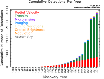
Figure 1.1. Exoplanet discoveries Credit NASA
The total exoplanets discovered over the past twenty years has risen dramatically – Figure 1.1. As can be seen the majority of these have been discovered by the transit method.
Transits occur when the planet crosses the face of the star from our line of view, causing a small but measurable dip in the star’s brightness. The key points in a transit needed to measure timing are shown in Figure 1.2. Ingress starts at t1 and by t2 the planet is fully within the stellar disk from our perspective. This is reversed for egress at t3-t4. The curve in the transit is caused by the change in brightness of the star from its centre to its limb, the limb darkening, and is different for every star and filter colour used.
![]()
Figure 1.2. An exoplanet transit
Exoplanet transits are explained in more detail by Paul Anthony Wilson here.
2.0 Why observe exoplanets?
With so many planets discovered detailed follow-up observations of only a very small percentage of these is possible with professional telescopes. Amateur observers can thus make a real contribution to exoplanet research by making such observations of known transiting exoplanets.
The regular measurement of transit times can be used to infer the presence of other unseen companion planets through transit timing variations (TTV’s). Measurements over long periods can reveal minute changes in a planets orbital period which may be due to orbital precession or even decay as planets follow a slow spiral into their host. Thus, these observations provide information the formation and dynamical history of the planetary systems.
Monitoring of exoplanet host stars is also important. Many host stars are active and magnitude measurements of the star can reveal the rotation period due to stellar spots. This has important consequences for the long dynamical stability of the planets and can indication interaction between the planet and star for very short period massive planets. Furthermore these measurements can reveal stellar activity cycles, not unlike the Sun’s 2 year cycle which impact on precision transmission spectroscopy used to determine the planet’s atmosphere. Therefore knowledge of these cycles can be used to inform the timing of observations large ground or space based telescopes.
The above are all good scientific reasons to observe transiting exoplanets but don’t lose sight of probably the most important reason, the shear fun of observing another world as it orbits its own star not to mention the chance to push yourself and our equipment to it’s limits.
3.0 What equipment is required?
Almost any instrument, typically available to amateurs, can be used for transit photometry – from a DSLR camera with a telephoto lens to a 400 mm Schmidt Cassegrain telescope. Figure 3.1.
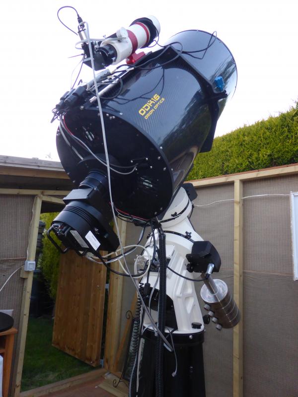
Figure 3.1 400mm Orion Optics ODK telescope with an ST10XME camera and an Astrodon Rc filter.
Obviously greater aperture allows fainter stars and smaller planets to be observed but many transits around relatively bright stars reach 3% depth, well within the reach of even modest telescopes. As the star needs to be observed continuously for 3+hrs a good solid mount with accurate tracking is essential. Ideally use a cooled monochrome CCD camera. If you are using a German equatorial mount it is possible that a pier flip will be required during the observations. Try to time these so that they don’t occur during the critical ingress/egress phases. Accurate time stamps on your data is vital so it’s important to use a dedicated software package such as the freeware Dimension 4 to update your PC’s clock at the start of every session and then at frequent intervals during the night. Don’t rely on your computer operating system to do this for you.
4.0 Which systems make good targets?
A good class of planet to start observing are the transiting Hot Jupiters. Being close to their host star many have short periods, so transits occur frequently and are of short duration. A list of such planets can be found on at exoplanets.org
– Select Table
– in the Example Tables and Save drop down box select Hot Jupiters – Figure 4.1
– To select by Orbital Period for example click on that column heading
– Data for the planet and star can be obtained by clicking on the planet name in the left-hand
column
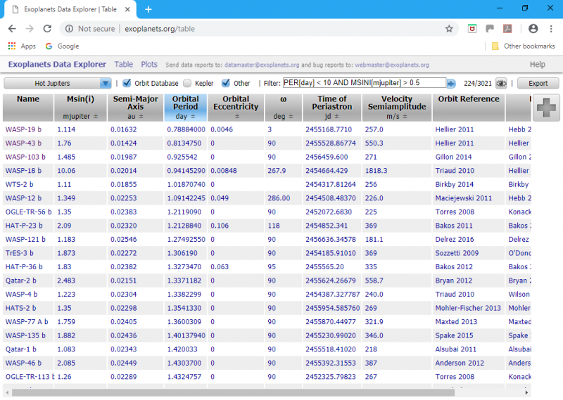
Figure 4.1 Screen shot showing a list of Hot Jupiters on the exoplanet.org database
This method requires some sorting to determine which planets are available for observation at your location. A simpler method is to use the transit predictor on the Exoplanet Transit Database (ETD). To list suitable targets, select Transit Predictions and enter your East Longitude and Latitude and click on Submit you are presented with a list of systems that transit on the selected night – Figure 4.2. It shows all systems with transit mid times for objects above 20˚. Note that times are in UT so you will need to make adjustments for your particular time zone and BST/Daylight Saving when applicable.
How to decide which exoplanet candidates to observe by Paul Anthony Wilson which uses data from the exoplanets.org website may also be of help in choosing a suitable target.
Other options which provide much greater control, but are a little more complex to use, are the Transit Ephemeris Calculator and the Transit and Ephemeris Service.
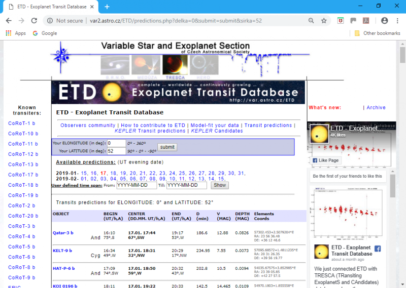
Figure 4.2. Screenshot showing predictions of transiting exoplanets for a given location
Selecting an exoplanet from the list on the left shows data for that planet and, by scrolling down, transit light curves. A specific light curve and associated data can be selected by clicking on TRESCA under the name of the submitting astronomer as in this example by Mark Salisbury – Figure 4.3.
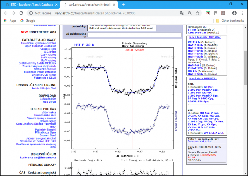
Figure 4.3. Screen shot of transit light curve of HAT-P-32 b by Mark Salisbury
5.0 A typical observing session
5.1 Planning
When planning observations is that it is important to obtain photometry either side of the expected start and finish time, transits may occur many minutes earlier or later than expected. This out of transit data can be used by software to detrend your data due to, for example, changing airmass. A good rule of thumb is to observe for half the expected transit duration either side of the expect start and finish times, though this is not always practical so aim for as much out of transit coverage as possible.
5.2 Imaging
Once you have a plan and a clear night you can set up to observe your target transit. To obtain the time series photometry you need a continuous series of images each of a few seconds to a few minutes’ duration. The time between the start of consecutive images is known as the cadence and includes the exposure duration and time between exposures for image download. A suitable cadence is governed by two factors, the signal to noise ratio (SNR) achievable for the target with your set up and the duration of the fastest changing portion of the transit which is the transit ingress/egress. An SNR of around 400 is ideal and most transit ingress durations are 10-30 minutes duration. A rule of thumb is to try and obtain 6-10 measurements during this ingress/egress duration. Before and after transit It is generally better to have slightly fewer measurements of higher SNR than more measurements of low SNR as this reduces the scatter in the photometry allowing more precise timing measurement but 30 mins of imaging during both of these periods should be considered the minimum. Uncertainty in the predicted ingress/egress times may dictate a longer period of imaging before and after the transit. Ensure that the counts per pixel for your target and planned comparison stars stay within the linear response of your CCD camera. The exposure duration must the same for all images in the time-series so take into consideration the effect of changing airmass during your observation before starting. If you find a star approaching saturation on your CCD as it rises then it’s better to slightly defocus rather than change the exposure duration which must remain the same throughout the exposure sequence. Analysis software can handle small focus changes using the FWHM tracking capability to determine photometric aperture sizes.
Following the same target for many hours requires good tracking and guiding. Because every pixel in a CCD camera responds slightly differently the highest precision photometry requires the star stays on the same pixels for the duration of the observations. This is very demanding and rarely achieved, even in professional observatories, so aim to keep movement of the star to the minimum possible.
One aspect that can be relaxed for precision photometry is focus, in fact the highest precision photometry is often achieved with stellar FWHM in the region of 10 arcseconds. Defocussing spreads the starlight over many pixels reducing the impact of pixel to pixel variations but there is a cost in increased exposure durations and difficulties for on-axis guiding. Even slightly out of focus stars can lead to improvements in photometry precision providing the SNR values can be maintained. For the very brightest stars defocussing is often essential to prevent saturation of the CCD.
For simple timing measurements unfiltered observations can be used but if you intend to combine your data with that from other observers or are working as part of a pro-am collaboration you should use a standard filter (a pro-am project will often define a preferred filter set). Stellar limb darkening gives Exoplanet transits different shapes and depths in different filters. I would recommend a photometric standard red filter such as Cousin Rc or Sloan r’. A clear-blue-blocking (CBb) filter can also be used, though it’s not considered a standard. All filters will slightly reduce the amount of light reaching the CCD requiring longer exposures but the red filters introduce a number of other benefits. A red filter helps minimise the effects of scintillation (twinkling stars) and provides better defined ingress/egress transitions allowing more precise transit timing measurement. The use of a filter also reduces systematics introduced by differences in comparison star colour from your target.
For transit timing it’s vital your camera control software accurately records the exposure start time and duration as these will be used by the photometry software to calculate exposure mid-time used as a timestamp for each image.
Obtaining high quality calibration data is one of the most important aspects of an exoplanet observing session. To achieve the best possible results, it’s important that your science images are properly calibrated with bias, dark and flat field correction in a standard fashion with the calibration frames obtained at the same CCD temperature as the science frames. You can never have enough calibration data so gather as many frames as you can (20+ of each is good). The individual frames should be median combined to create the master calibration files before application to your data and always keep copies of the originals in case something goes wrong. The BAA photometry manual can provide good advice on obtaining and using calibration data to produce high quality photometry.
6.0 Producing a light curve
If everything has gone well and the weather has been kind, you should now have up too few hundred science images and associated calibration data it’s time to turn them into a transit light curve. For this we recommend using AstroImageJ (AIJ), a data reduction and photometry package that is both free and designed specifically for exoplanet transits. It can appear a little daunting at first but there are a lot of good resources available to help as detailed on the BAA Exoplanet Division website’s Guides/Tutorials page.
Figure 6.1 shows a transit observation of WASP-52b obtained from the UK on 2nd November 2018 using a 400mm Orion Optics ODK telescope with an ST10XME camera and an Astrodon Rc filter. The black dots are the photometric measurements obtained from AstroImageJ using the process described in the text. The red line is the best fit transit model from ETD. WASP-52b is an excellent target for observing, orbiting its 12th magnitude star every 1.75 days producing a transit with a depth over 3%. Note the strong limb darkening effect visible as the curvature in the curvature in the base of the transit. This effect is strongest at shorter wavelengths (blue) and smallest at longer (redder) wavelengths, highlighting the importance of filters
![]()
Figure 6.1 Transit light curve of WASP-52b Mark Salisbury
Figure 6.2 shows a phase folded transit light curve of HAT-P-23b.The original data (grey dots) consists of 1755 data points taken from 11 transits observed with the Open University 17.5” PIRATE telescope at the Observatorios de Canarias on Mt Teide on Tenerife and a further 6 transits observed by author using his 16” UK based telescope. The black dots represent bins of 25 data points and the red line is the best fitting transit model from Exofast. The out of transit residuals of the binned data to the Exofast model are just 390 parts per million, comparable to a single observation from a 2m class telescope.
![]()
Figure 6.2. Phase folded observations of HAT-P-23b. Mark Salisbury
The data processing module within AIJ provides quick and simple standard data reduction including updating FITS headers and plate solving, which considerably simplifies the photometry process. The process for photometry in AIJ is covered in depth in the available literature but it allows you to simply fit a physical model of the transit to your data which can then be used to assess the quality of the photometry. To create a model fit all you need to start with is the orbital period, the stellar radius and the limb-darkening parameters. The former can be obtained from one of the many online catalogues, the limb-darkening can be obtained using the calculator found on the Exoplanet Utilities website. Within the AIJ photometry module you enter your camera parameters and then select as many comparison stars as possible that are of similar brightness to your target, ensuring none are known variable stars. For ensemble photometry AIJ will create an aperture template. After you have run the photometry take a note of the RMS residual and BIC values from the model fit and try the photometry again varying the aperture settings until you find the settings that minimise both values. This is where doing the plate solve pays off as AIJ will automatically apply your template again and will follow the stars even through a meridian flip making this a quick and simple process. AIJ also provides an option to vary the photometry aperture based on the FWHM of each image. The software then allows you to step through the comparison stars removing them one at a time to see if any are adding excessive noise to the light curve, again looking the minimise the RMS and BIC values leave out any comparison stars that increase these values significantly. Finally follow the steps outlined in the AIJ documentation to save your data in the format you want.
7.0 Sharing data
Now you have your transit light curve you should share it. It is recommended that you upload your data to;
a) The BAA Photometry Database Figure 7.1
A login is required and User Guides are available via the Help and Notes on Submitting Observations buttons. Data is uploaded to the AAVSO database quarterly.
b) The Exoplanet Transit Database (ETD) – Figure 7.2
Data is input via the Transiting ExoplanetS CAndidates (TRESCA) project – Figure 7.3. Observers can register using the link on this page.
Amateur results submitted to the ETD have created a rich data set. This data has been used by researchers in many peer reviewed journal papers.
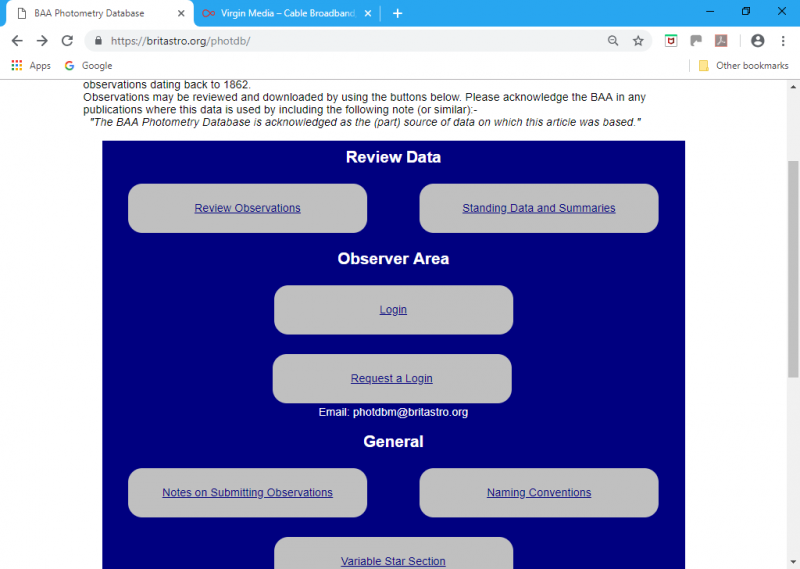
Figure 7.1. Screenshot of the BAA Photometry Database homepage
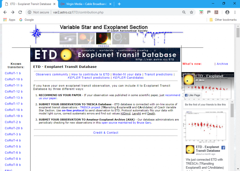
Figure 7.2. Screen shot of the ETD homepage
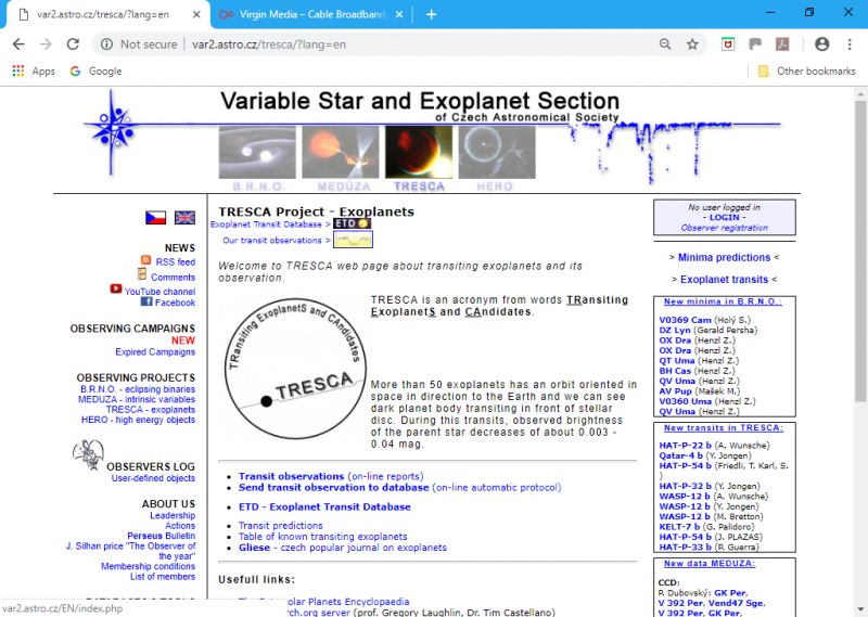
Figure 7.3. Screenshot of TRESCA project homepage
8.0 Resources
8.1 Websites
Access the Guides/Tutorials page on the BAA Exoplanet Division’s website for help with
AstroImageJ and other aspects of target selection, imaging and analysis
8.2 Books
Listed on the Publications page in particular;
Transiting Exoplanets by Prof. Carole Haswell published by Cambridge University Press, 2010,
£31.99 (Paperback). Also used in the Open University S382 Astrophysics module
The Exoplanet Handbook by Michael Perryman published by Cambridge University Press 2018,
£56.99 (Hardback)
Edited by Roger Dymock
https://britastro.org/wp-content/uploads/2019/02/MS-scope.JPG
| The British Astronomical Association supports amateur astronomers around the UK and the rest of the world. Find out more about the BAA or join us. |