2019 June 16
Observing the outbursting comet 29P/Schwassmann-Wachmann
Background
Of all the known objects in the Solar System, Comet 29P seems to be the least well-understood in that it is in a continuous state of activity, intermittently exhibiting single, double or multiple outbursts quite unlike any other comet. The name ‘comet’ may mislead you to think it makes the occasional close visit to our neck of the woods and becomes active as it nears the Sun, sporting a tail as it does so. The reality couldn’t be much further from this! Here’s an image showing its unusual appearance (Fig. 1):
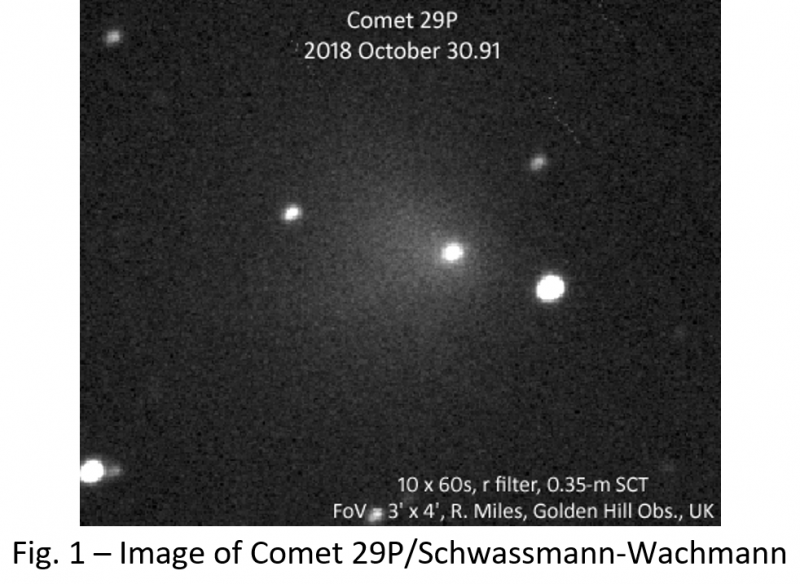
You can see a diffuse coma, the result of a series of multiple outbursts that ended 3 weeks earlier, together with a bright stellar ‘nucleus’ generated by a new outburst that occurred just 36 hours before the featured image was captured.
Researchers believe this object has remained in the trans-Neptunian region as an inert body for billions of years, before more recently being gravitationally perturbed by Neptune, Uranus, etc. and that it is now displaying intermittent outbursts, typically 10 per year, whilst temporarily trapped in a near-circular orbit between the giant planets, Jupiter and Saturn. See how its current orbit compares:
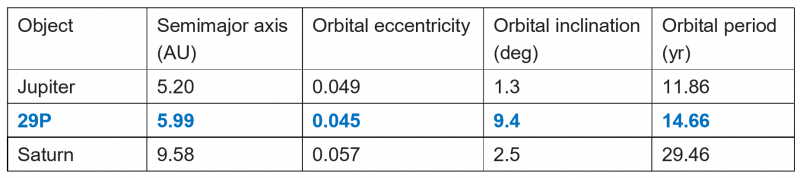
Although vastly smaller than the planets, 29P is very much larger than a typical comet and even larger than Comet Hale-Bopp. Being much more distant than main-belt asteroids, the apparition of this ‘mini-planet’ comes around every 392 days (rather like Jupiter does) and it is visible far enough from the Sun in the sky for ~310 days at a stretch. Given it is visible for about 80% of the time, it is an ideal observing target and our aim is to monitor its activity in as much detail as possible to better understand its true nature. How then do we go about this?
How to observe comet 29P
You will need a fairly large telescope, say at least 15-cm aperture (the larger the better!) and a focal length of >100 cm, as well as an image scale for your camera of preferably <2.0 “/pixel. Use a monochrome camera, and take a series of exposures using either no filter, a Luminance filter, or a red filter. I like to use an exposure time of 60 sec but if your mount does not track well then shorten the duration to say 20 or 30 sec as the objective is to stack the images to create a higher quality stacked frame for measuring.
Stacking individual frames
As to how many images you can stack without undue trailing, that depends on the apparent rate of motion of the comet across the sky, which never exceeds 0.52 “/min, as well as the apparent size of stars recorded by your camera. If the atmosphere is fairly steady, the latter may typically be about 2.5” in size (called the Full-Width at Half Maximum intensity, or FWHM). The advice here when stacking is not to trail the comet or stars by more than 1 x FWHM, which means all of the tracked frames should span a time of no more than 2.5/0.52 = 4.8 minutes in the worst case, i.e. say 4 x 60 sec stacks. Now this is important: you should check what the apparent speed of 29P on the date you observed before stacking frames. You can do this by going to the Minor Planet Ephemeris Service at: https://www.minorplanetcenter.net/iau/MPEph/MPEph.html
Enter ’29P’ in the box, and the date (e.g. in format, YYYY MM DD), in the ‘Ephemeris start date’ box, and ‘1’ in the ‘Number of dates to output’ box. Then click on ‘Get ephemerides/HTML page’ and you will see the values you need under ‘Sky Motion’ in units of “/min as well as the direction (P.A.) of motion in degrees.
By taking the trouble to find out the apparent speed and direction the comet moves, allows you to stack your frames in a cleverer way than most people adopt!
Use stacking software that permits you to enter the apparent motion and P.A. direction – Herbert Raab’s software Astrometrica is a good choice for doing this, as well as for plate solving and making astrometric and photometric measurements. (Astrometrica has a tutorial option to get you started using the software). The ‘trick’ now is to track and stack at ONE HALF the apparent speed in the SAME P.A. direction as the moving object. This then trails both the mover (29P in this case) and the stars in equal measure. So now the above scenario in 2.5” FWHM seeing is for the tracked frames to span a time of no more than 2.5/0.26 = 9.6 minutes in the worst case. N.B. This doubles the number of frames you can stack without undue trailing, and also ensures that the appearance of the moving object on the stacked image is the same as the stars, which increases the accuracy of the photometry.
Here’s how you produce “tracked and stacked” frames in Astrometrica for subsequent analysis:
Click on ‘Astrometry’, ‘Track & Stack…’, ‘Add’, and then select the image frames you wish to combine to produce a good signal-to-noise stacked image for measurement. Then click on ‘OK’ and the software will load those frames into memory and a new dialogue box appears entitled ‘Coordinates, Tracking and Stacking’. Make sure the coordinates in the ‘Right Ascension’ and ‘Declination’ boxes are close in value to those of the centres of the image frames used to stack so that the software can identify the reference stars and solve the image. Then under
”Coordinates, Tracking and Stacking ‘, ‘Object Motion’, ‘Speed’:- Enter the apparent speed of 29P in “/min divided by 2
”Coordinates, Tracking and Stacking ‘, ‘Object Motion’, ‘P.A.’:- Enter the direction of motion in degrees
These values are available at: https://www.minorplanetcenter.net/iau/MPEph/MPEph.html
”Coordinates, Tracking and Stacking ‘, ‘Stacking’:- Click on ‘Average’ then on ‘OK’
You then save this “tracked and stacked” image by clicking on ‘File’, ‘Save as FITS… ‘, ‘Save’
N.B. For photometry, it is well worth stacking two or more images and saving the file for separate analysis. The main reason is the improved signal-to-noise in the image, which then increases the number of usable reference stars and hence improves accuracy. Astrometrica also saves an accurate value for the R.A. and Dec. of the centre of the stacked image in the FITS header making subsequent plate solving a doddle.
[Warning: If you try to do photometry on the initially-stacked frame, Astrometrica only uses the reference stars from the first image in the series to calibrate the photometry (zeropoint calibration). If the sky transparency happened to vary during the time series then the first frame will not be representative of the average of all the frames and this will introduce a bias error in the photometry.]
Performing photometry
Although Astrometrica was written primarily for doing Astrometry, it has been improved over recent years and now permits Photometry to an accuracy of 0.02 magnitudes or so. To achieve this, you have to use a different Settings configuration than when reporting Astrometry. For 29P, we have standardised on some settings so that everyone’s measurements are largely equivalent. Here’s what is important when setting up the configuration for accurate photometry of “tracked and stacked” images of 29P:
Using Astrometrica Version 442 or later, go to ‘Settings‘, then under the tabs:
‘Observing Site’, ‘Location’, ‘MPC Code’:- Enter the IAU Code of your observatory or ‘XXX’ if you do not have a Code
‘CCD’, ‘Time in File Header’:- Usually this is set to ‘Start of Exposure’, but click ‘Middle of Exposure’ if you are using an Astrometrica-stacked frame (see below)
‘CCD’, ‘CCD Chip’, ‘Saturation’:- Enter ‘40000’ if your max. pixel value is 65535
‘CCD’, ‘Color Band’:- Click ‘Red (R)’. This operation ensures that the analysis yields the Cousins R magnitude, also referred to as the Rc magnitude.
‘CCD’, ‘Color Band’, ‘Filter’:- Select ‘Clear/None’ from the drop-down menu if you have not used a filter or have used a Clear/Luminance filter; or if you have used a red filter then click ‘R (Cousins) ‘ or ‘r’(Sloan) ‘ as appropriate. This operation ensures the filter has been identified and is logged in the Photometry file as ‘C’, ‘R’ or ‘r’.
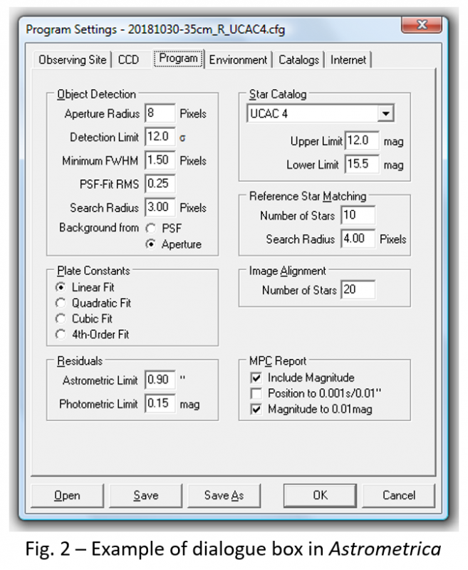
‘Program’, ‘Object Detection’, ‘Aperture Radius’:- Here you have to select the size of your photometric measuring aperture in pixels. This is a crucial step as we try to utilise a standard value for the measuring aperture in terms of arcseconds (“) on the sky. Since everyone has different telescope focal lengths / cameras / binning, this means you have to know what 1 pixel in the image subtends by way of angle on the sky. This should be as close as possible to 5.65”. Take my own setup, with a focal length of 2731 mm and 4.5 μm square pixels, when I solve an image, the Log File gives a Pixel Size of 0.68”, so the Aperture needed for photometry measures 8 pixels (5.44”) radius. As your setup will be different, pick a number of pixels that comes in just under the standard of 5.65” if you can. (N.B. Short focal lengths may force you to use the minimum of 3 pixels radius to stay close to the optimum).
‘Program’, , ‘Object Detection’, ‘Detection Limit”:- A value of ’12’ is suggested to ensure that brighter stars are used in the plate solution, also speeding up the analysis in the process.
‘Program’, ‘Object Detection’, ‘Background from’:- Click on ‘Aperture’
‘Program’, ‘Plate Constants’:- Click on ‘Linear Fit’
‘Program’, ‘Residuals’, ‘Photometric Limit’:- Enter ‘0.15’ mag
‘Program’, ‘Star Catalog’:- Select ‘UCAC 4’ from the drop-down menu. This star catalogue incorporates the AAVSO’s All Sky Photometric Survey (APASS), which has accurate photometry for stars brighter than about magnitude 16.
‘Program’, ‘Star Catalog’, ‘Upper Limit’:- Enter ‘12.0’ mag
‘Program’, ‘Star Catalog’, ‘Lower Limit’:- Enter ‘15.5’ mag
‘Program’, ‘Reference Star Matching’, ‘Number of Stars’:- Enter ’10’
‘Program’, ‘MPC Report’:- Click on ‘Include Magnitude’ and ‘Magnitude to 0.01 mag’
‘Environment’, ‘Directories’:- Enter the same directory for ‘CCD Images’ and ‘Output’
‘Catalogs’, ‘UCAC-4’:- Click on ‘VizieR’
After producing one or more sets of tracked and stacked images, you can undertake photometry on each. Do first check before you start that under the tab, ‘CCD’, ‘Time in File Header’ you have selected the ‘Middle of Exposure’ option when working with stacked frames. N.B. You do not need to analyse single frames or stacked images one by one, as you can load up to 25 at any one time in Astrometrica. Do this by selecting ‘File’, ‘Load Images…’ and selecting the stacked frames you wish to analyse. Then click on ‘Astrometry’, ‘Data Reduction… ‘ and ‘OK’. If successful, a new dialogue box entitled ‘Data Reduction Results’ should appear at the lower right (this is also shown in the lower part of Fig. 3).
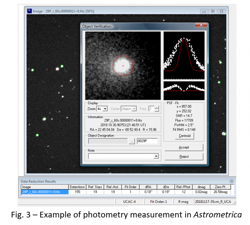
[A hint: For the “plate solution” to be reliable, the number of stars used for photometry (listed under the heading, ‘Ref/Phot’) should be between 50% – 80% of the total number of reference stars identified (listed under the heading, ‘Ref. Stars’). To adjust the proportion of stars used for photometry, you should try altering the 0.15 mag photometric limit in the Settings, i.e.:
‘Program’, ‘Residuals’, ‘Photometric Limit’:- Enter ‘0.15’ mag
Also, the photometric precision achieved by the fit can be judged from the value listed under the heading ‘dmag’: in the Fig. 3 example, this is 0.02 mag].
Now position the cursor on or very near to the brightest part of the image of 29P and click. A new dialogue box entitled ‘Object Verification’ appears (shown in Figure 3) depicting the astrometric and photometric results. The red circle shows the actual size and position of the measuring aperture so make sure this is centred on the pseudo-nucleus of the comet. You then enter ‘0029P’ in the unlabelled box as shown, and then click ‘Accept’. Although nothing appears to then happen, in actual fact 3 output files are created and the contents of these can be accessed by going to:
1. ‘File’, ‘View MPC Report File’, which lists the astrometric results together with photometry to the nearest 0.01 magnitude. These data, which are set out in MPC report format, are the end result of the exercise.
One point to note is that if your observatory has an IAU Code and you want to report your results to the Minor Planet Center, you will have to edit the individual measurement lines by changing the magnitude values from 2 decimal places to 1 decimal place as shown:
0029P C2018 10 30.91470 22 45 03.94 -00 52 49.5 15.96R J77
=> 0029P C2018 10 30.91470 22 45 03.94 -00 52 49.5 16.0 R J77
You then send that report as an ASCII file to obs@cfa.harvard.edu
2. ‘File’, ‘View Photometry File’, which now lists the mid-time of the observation as the corresponding Julian Date, the derived magnitude to a precision of 3 decimal places, the signal-to-noise ratio of the target, the zeropoint value of the calibration, and the catalogue used.
————————————————————————–
JD mag Flt SNR ZeroPt Cat Design.
————————————————————————–
2458422.41470 15.960 R r 111.35 26.610 UCAC4 0029P
—– end —–
3. ‘File’, ‘View Log File’, which lists a vast amount of information underlying the astrometric and photometric plate solutions. Rather than go into any detail here, I recommend you peruse this text file after having carried out an analysis as that will give you a further understanding of how Astrometrica works.
Reporting photometry of 29P
The above approach yields the brightness of the pseudo-nucleus combined with that of the inner coma out to a radial distance of ~22,500 km. This quantity is sometimes referred to as the nuclear magnitude, or m2 magnitude, and in the case of 29P is very sensitive to cometary activity on its nucleus.
Fig. 4 illustrates the observed photometric behaviour of 29P during its latest apparition of 2018–2019. Here the measured R magnitudes have been normalised to what they would have been if situated 1 AU from the Sun and seen from the Earth at a distance of 1 AU. The phase angle has also been corrected to a value or 0 degrees using a 0.035 mag/deg phase coefficient.
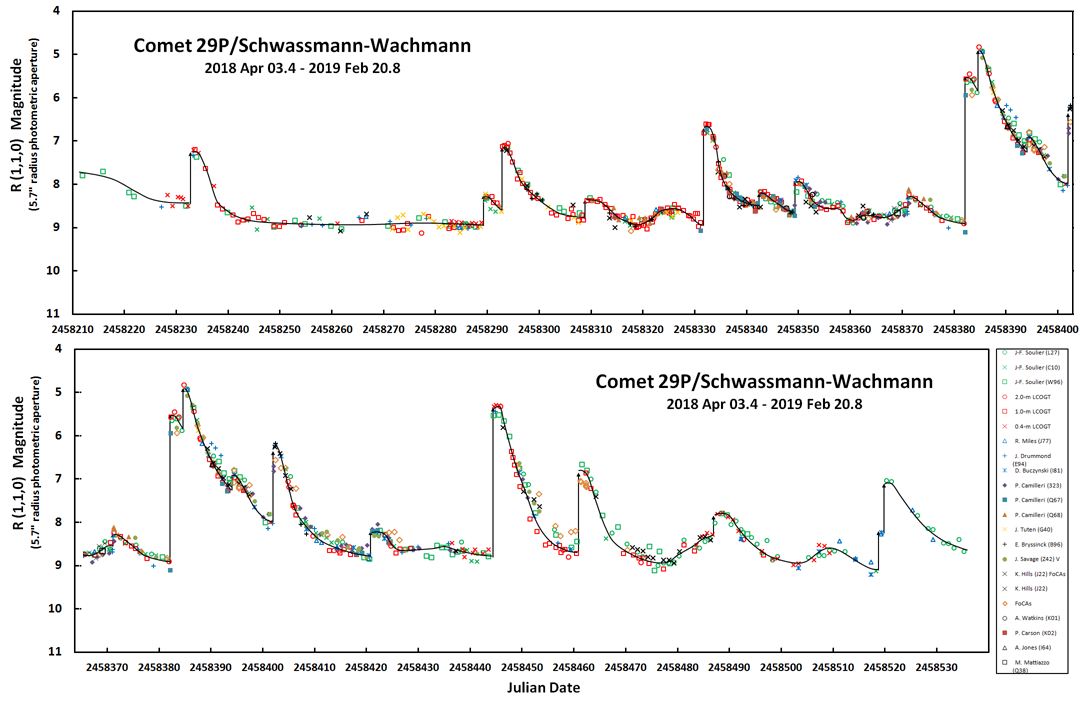
Note the very sudden changes in brightness of up to 4 magnitudes (a factor of 40) caused by outbursts of the nucleus. Most of the rise to maximum occurs within the space of 1 hour or so and therefore is rarely observed. During an apparition, which lasts for up to 11 months, the comet describes only a relatively short arc in its orbit around the Sun. An entire orbital year requires some 15 Earth-years and so it is essential that we continue to monitor 29P year on year so that we can study the seasonal changes in its behaviour. The comet is currently moving northwards in the constellation of Pisces and so should be readily visible to northern hemisphere observers for the next 5-10 years.
Results should be reported to the author via the baa e-mail address, ‘arps@britastro.org’ or my personal e-mail address, and images to the Comet Section via ‘cometobs@britastro.org’. If possible, report your results in MPC astrometric format expressing the R magnitude to 2 decimal places. Additional information in the form of the Photometry File data would also be helpful. Observations with or without a red filter are equally valuable.
Download the article as a pdf here.
Richard Miles
2019 June 8
| The British Astronomical Association supports amateur astronomers around the UK and the rest of the world. Find out more about the BAA or join us. |