B.A.A. GUIDE TO OBSERVING JUPITER                 

John Rogers (Section Director), 2026 July

[A PDF version of this Observing Guide is available here:]  BAA observing guide_Jup-for-web_2026july_final&figs

Introduction: Why observe Jupiter?

Jupiter is the largest of the planets. For most of the time it is also the one with the largest disk, the most detail, the most activity – and the greatest opportunity for real scientific contributions by the BAA. The planet and its satellites provide an endless source of interest for even a casual observer. For the more serious observer, we are continuing a long-term programme of observation which still has not exhausted all the important phenomena that the planet can display, and which is valued by professional scientists. Observations by spacecraft or professional observatories complement but do not replace our data.

Jupiter orbits round the Sun once in about twelve years. It is therefore at opposition (highest altitude at midnight) at intervals of about thirteen months. Its apparent diameter does not vary greatly, so it can be observed for much of the year. Even binoculars will show the four largest satellites. A small telescope will show that the planet’s disk is divided into dark belts and bright zones, which extend along parallels of latitude. A telescope of 80mm aperture or greater will reveal irregularities, mottlings, and spots of various kinds along the belts and the zones. These spots move visibly within ten minutes, carried round by the planet’s rapid rotation; it rotates about 2.5 times per terrestrial day. All the visible features are clouds in Jupiter’s thick atmosphere, and the rapid rotation is responsible not only for the evident polar flattening, but also for the characteristic motions of the spots from day to day, which run almost entirely parallel to the belts and zones. Thus, different latitudes have slightly different rotation periods.

Our aims are to monitor the currents, colours, and disturbances in the planet’s atmosphere, and to produce scientifically valuable reports on them. It was largely the work of BAA members that established the normal currents and the types of disturbance to which they are subject. It is still necessary to measure the motions of spots, so as to identify which of the known currents they belong to, and to look for unusual interactions. This is a prerequisite for studying their individual properties and their place in the overall behaviour of the jovian atmosphere. In addition, modern imaging provides new insights into the meteorological processes involved.  Sometimes we record dramatic outbreaks that develop over days or weeks; we also record patterns of activity that may develop and change over years or decades (Figure 1).

We recognise that many observers will be satisfied with simply seeing the features on this splendid planet, and this guide gives some tips to doing so effectively.  But the data that we use for analysis is now almost entirely from images, which nowadays show much more detail than  can be seen visually. The planet as seen by eye has lower contrast and a more subtle range of colour (mostly shades of yellowish-brown), so when you first look at the planet, you may see less than you expect.  But after spending some time getting accustomed to the view, especially in good seeing, you will begin to pick out more features and detect colour differences between them, and to track them across the disk as the planet rotates. Even observers mainly interested in imaging should know what the planet looks like visually, so that they are not led astray by the endless possibilities in image processing.

Observing is always more interesting, and potentially useful, if you know what you are looking at. So we start with a brief outline of what can be seen, and the names that we use to describe features.

The most obvious features are the belts and zones, whose names and abbreviations are shown in Figures 2 & 3 (and their captions).  The names were originally defined for the visibly dark belts and bright zones, and are still used thus by observers. However, sometimes one or more of the dark belts may be missing, in whole or in part, and sometimes there may be extra belts or components of belts. Indeed, in the high latitudes beyond the NNTB and SSTB, there are few if any distinct belts.  But thanks to spacecraft, we now know that the visible bands are bounded by a regular pattern of jet streams in fixed latitudes (Figure 2), and this has enabled us to adapt the traditional nomenclature in a precise way according to latitudes.  The eastward (‘prograde’) jets form permanent boundaries between ‘domains’ formed of a belt (cyclonic, at lower latitude) and a zone (anticyclonic, at higher latitude), and the visible belts and zones always revert to these positions even though they may vary temporarily. An observer can usually refer to the belts and zones by their traditional names and appearance, but in case of ambiguity, their identity can be established from their latitudes, which can only be measured accurately from images. When one of the standard belts is seen to be double, the two components are indicated by N and S in parentheses, e.g. SEB(N) and SEB(S); the space between them, in this example, is named SEBZ. Suffixes, as in SEBn and SEBs, have also been used to denote belt components but we now reserve these to denote belt edges. A Band is a narrow dark belt within one of the standard zones, e.g., EB (Equatorial Band) in the EZ.

Observers with moderate-sized telescopes can see most of the important cloud features on the planet and can track their movements and developments. Major upheavals, occurring every few years, can include whitening then revival of the SEB (‘SEB revivals’) or the NTB (‘NTB revivals’), and comparable cycles of the NEB (‘NEB broadening events’) (Figure 1). Each of these produces impressive arrays of rapidly-changing spots.  A zone, notably the EZ, may develop strong colour for a year or more.  Conspicuous local features usually include the Great Red Spot (GRS) (although it has been shrinking), and the NEBs dark formations (NEDFs), while higher resolution can reveal white ovals and other features in various latitudes.  Spacecraft imaging has shown that many features that were visually diverse or ill-defined actually belong to a small number of meteorological types, and our observations now are giving better understanding of how those types behave.

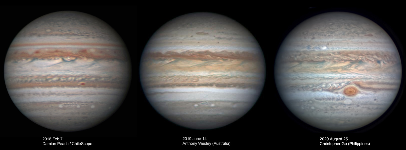
Figure 1.  Some of the best amateur images of Jupiter showing variations over 3 years (2018-2020).  Note the changing colour of the Equatorial Zone, and changing appearance of the NEB.  In 2020 (right), a NEB expansion event is in progress, and a brilliant white spot is initiating a NTB revival; the Great Red Spot is strongly red. North is up.  Images by Damian Peach (using 1-metre ChileScope), Anthony Wesley, and Christopher Go.

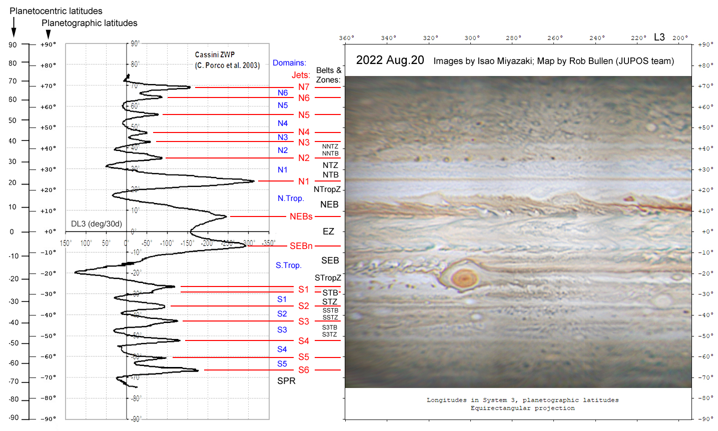
Figure 2.  Definitions of Jupiter’s jets, domains, belts & zones, aligned with a typical map from a BAA report (shown with north up).  On the left is a graph of wind speed vs latitude (zonal wind profile), from the Cassini flyby.  The prograde (eastward) jets are numbered in order, and the domains between them are given the same number as the jet on their equatorward side.  Within the lower-latitude domains are the traditionally named belts and zones, named with the following abbreviations: B, Belt; E, Equatorial; N, North; S, South; T, Temperate; Trop, Tropical; Z, Zone. GRS, Great Red Spot; NPR, North Polar Region.

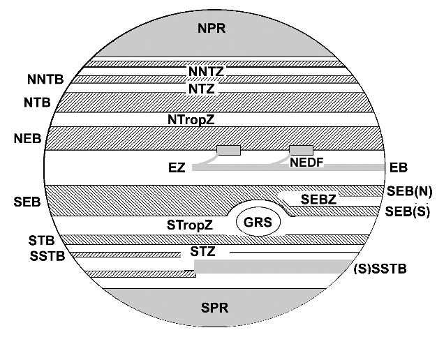
Figure 3.  Diagram showing the standard positions of the belts and zones, named as in Figure 2. On the right are examples of typical variations and features (GRS, Great Red Spot; NEDF, NEBs dark formation).

Coordinate systems

The coordinate systems used for locating features on Jupiter are, unfortunately, complicated: partly due to the planet itself, and partly because the systems that were defined over a century ago have been superseded by different systems in professional usage – so we now have to accommodate both.  So, as the planet was usually viewed with an inverting telescope in the northern hemisphere (as you may still do), pictures of it were always presented with south up; but the present convention requires north up, so that is what we show in our reports.  Because Jupiter’s profile is elliptical (oblate), there are two systems of latitude, called planetographic (which we and most other groups use) and planetocentric (used by NASA’s Juno project). For longitude, as there are no fixed reference points on the planet’s surface, three arbitrary longitude systems have been defined, with exact rotation periods chosen to be close to the average periods for important features: System I (9h 50m 30.003s, for the equatorial region), System II (9h 55m 40.632s, for the Great Red Spot etc.), and System III (9h 55m 29.711s, for the planet’s magnetic interior).

Longitudes are abbreviated as L1, L2 or L3, and central meridian longitudes as CM1, CM2 or CM3. (In the past we used greek lambda and omega respectively for L and CM.)  System I is used for near-equatorial features between ~10ºN & S, and System II for other latitudes, while System III is required in all professional work and in our maps.

The observer should record the exact time to which any observation refers (preferably to the nearest 0.1 minutes for images), and calculate CM1, CM2 and CM3 for it.  These should be obtained from the WinJUPOS program (which is available free at http://jupos.org), or from the tables in the BAA Handbook. The Handbook gives the CM longitudes at 00h UT on every night, and tables showing the increase of longitude with time. All you need to do is to subtract or add the appropriate longitude increments so as to find the CM longitude at the time of each observation.

Visual observations

Major features such as belts and equatorial dark projections can be seen with an 80-mm telescope, but satisfactory observations require a telescope of at least 150mm aperture. For a beginner it is worth trying the following methods of observation, so that you can make useful records if they ever see anything unexpected on the planet. For those who want to make systematic visual observations, report forms can be downloaded from our website. Observations should be submitted to the Section Director every few months, or sooner if something novel or exciting is observed.

More detailed advice on drawings and other types of visual observation is still on the Jupiter Section’s older (pre-2015) web site at: https://britastro.org/jupiter/programme.htm. (However, please note: that web site is no longer maintained so links on it are out of date.)

Drawings: Most people like to draw what they see, and this is a skill that takes some practice to develop. Good drawings are worthwhile as illustrations of the general appearance of the planet (Figure 4), for comparison with records in previous centuries, and may sometimes be useful as records of special events. As with all serious observations,  it is essential to record only what you can see, and not be influenced by expectations, which is all too easy now that people are used to seeing high-quality images.  Before starting a drawing, inspect the planet carefully, including the widths and intensities of the belts and zones. Then make a quick outline sketch so that the main features are positioned at a single time, then fill in the fine details.  It’s worthwhile to add colour if there were different hues, and some observers will be able to  develop their style so as to combine observational accuracy with artistic quality.

Longitude measurements: The longitudes of spots can be measured by timing their ‘transits’; one just notes the exact time at which the spot crosses the CM. Any observer who sees an unexpected, possibly novel feature on the planet is encouraged to make a transit-timing and report it.  The observer should give the transit time to the nearest minute (which corresponds to 0.6º of rotation in longitude), and calculate the longitude. An advanced observer might find it interesting to make transits systematically through an apparition, which was how the Jupiter Section tracked features in the past, and then plot charts of longitude versus time to follow spots on their different currents over several months.

Colour and intensity estimates: Systematic verbal estimates of the colours of belts and zones may be useful, if made with a reflecting telescope or SCT of at least 250mm aperture. There are subtle long-term changes and sometimes dramatic short-term ones, as when a zone adopts a yellow colour. Although there is considerable scope for artefacts, g., due to subjective colour contrast effects, this is also true of colour images, due to use of different filters and image processing. Observers should familiarise themselves with the spurious colour effects that may be induced by the telescope (particularly refractors), the eyepiece, the eye, and the Earth’s atmosphere. (The ‘traffic-lights effect’ — fringing with red at top and blue-green at bottom –can apply to each zone as well as to the whole disk.) Colours are easier to discern in twilight.

Intensity estimates are made numerically, on the same scale as for the other planets, from 0 (brightest) to 10 (black sky). They are inevitably subjective, so are only worthwhile if done systematically and repeatedly. Observers who make colour or intensity estimates should tabulate and average them for the whole apparition, and note any significant changes.

Observations of satellite phenomena: The transits, shadow transits, eclipses and occultations of the four Galilean satellites are among the most striking phenomena that a beginner can observe. There are few other systems which demonstrate planetary motions so directly to the eye. Also, transits in front of the planet reveal the different surface brightnesses of the satellites themselves: Callisto and Ganymede very dark, Io pale, and Europa usually invisible against the bright clouds. (Surface markings, however, are rarely visible even with large telescopes.) Although observations of the satellite phenomena no longer have any scientific significance, observers may like to make accurate drawings of them, especially when several are occurring at once.

The phenomena of the satellites are predicted in the Handbook, and can be visualised using WinJUPOS.  Every six years, during a few months when the plane of the system intersects the Earth, the satellites can be seen to occult and eclipse one another in ‘mutual phenomena’.

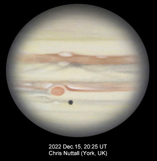
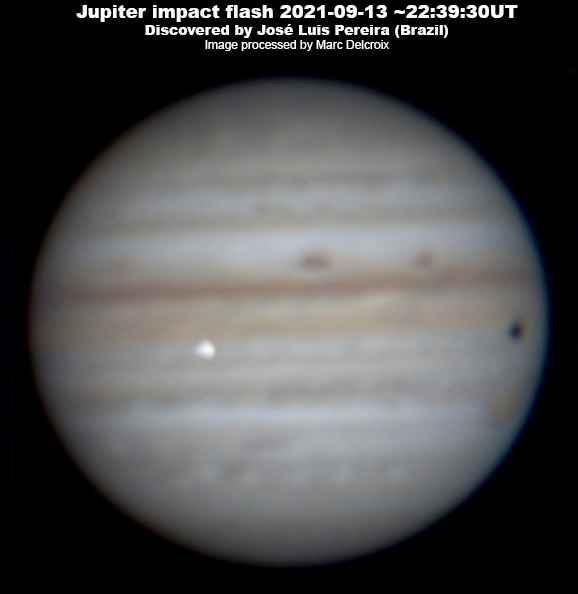
Figure 4 (L).  Drawing of Jupiter, by Chris Nuttall.  Note the shading which dims features near the limb (‘limb darkening’).  There is a satellite shadow on the SSTB, near the GRS.

Figure 5 (R).  Image showing an impact flash.  The flash only lasts 1-2 seconds, and may be distorted by the seeing, but the image was integrated over a longer interval to improve the signal-to-noise ratio.  Image by José Luis Pereira, processed by Marc Delcroix.

Digital imaging

In general any telescope of good quality can be used for imaging, with an aperture of at least 100mm for good-quality refractors, or at least 150mm for reflectors.  But telescopes of 200–400mm are needed for the very detailed images that are now used for the Jupiter Section’s analysis, from observers all around the world. Planetary imaging is now done using specialised planetary cameras (evolved from webcams) with CMOS sensors, which have superseded CCD sensors in recent years. There have been rapid improvements in the sensitivity and speed of such cameras which have particularly benefitted images of Jupiter.  The images provide an objective record with high resolution and good colour discrimination, and enable accurate measurements of both latitude and longitude.

The camera is used to capture many hundreds of images within a few minutes. Then, software such as Autostakkert! or (more recently) LuckyStackWorker is used to select and superimpose the best frames, omitting those where the resolution was degraded by the atmospheric seeing. Then a program such as AstroSurface or waveSharp (successor to Registax) is used to sharpen and enhance the resulting composite image.

Colour cameras are suitable for routine use.  An infrared blocking filter should be employed to ensure the image is not ‘polluted’ with infrared signal (since the detectors are sensitive up to 1.0 microns wavelength). Alternatively, images can be taken with a monochrome camera plus a set of colour filters: this allows the observer to obtain separate images in red, green, blue, and possibly IR and UV (see below). (Again ensure that unwanted IR signal is blocked, either by a separate IR blocking filter or by using IR-blocking-coated colour filters.)

Because of Jupiter’s rapid rotation, images composited over an interval of more than 2-3 minutes will be degraded by its movement.  However, there is a ‘derotation’ function in WinJUPOS and (more recently) in LuckyStackWorker which can reproject images to a fixed CM longitude.  This enables observers with mediocre seeing to select sharp frames from a longer interval, even tens of minutes, and produce a high-quality image.  It can even be applied separately to a transiting satellite or shadow, which can otherwise appear as an unsightly smear. (Incidentally, the best amateur images now routinely show visually elusive features such as Io’s bright equatorial band or Ganymede’s dark patches when in transit.)

Image processing is necessary to bring out the planet’s limb, and is desirable to enhance contrast and perhaps to sharpen features. Such image processing should be done judiciously with awareness of the artefacts that it can create; check that there are not conspicuous rings around satellite shadows, nor any saturated white areas in the image, and that the belt/zone contrasts are not lost.  Software with AI (‘Artificial Intelligence’) must not be used in processing images as it can distort or even invent details.

Images in different filters can be very informative as different levels in the atmosphere are seen. There is little variation across the middle of the visible spectrum, but deep blue (or violet) and red give good discrimination. Near-IR (~740-850nm) images look like extreme red-light images, and can show much small-scale detail as they penetrate some way into the main clouds, and are often less impaired by atmospheric seeing.

Some observers produce images with a separate luminosity channel (‘LRGB’ images); then it is essential to state what waveband is used for the luminosity channel, and normally this should be white.  Some observers use a near-IR image, which often has higher resolution than visible colour, for luminosity to create an ‘IR-RGB’ image; but these appear seriously unrealistic. A much better technique has been introduced recently using ‘IR wavelet decomposition’, in which the RGB colour channels are combined with the sharpness, not the luminosity, of an IR image [‘wIR-RGB’ images; see note in our Report 2025/26 no.4].

Observers with large telescopes can also take images in the ultraviolet (~360nm) and the methane absorption band (890nm), which reveal the high hazes in the atmosphere; these require longer exposures. These images must not be over-processed as the relative intensities of features are more important than fine detail. Methane-band images highlight high-altitude features such as long-lived anticyclones or brief convective outbreaks.  Many observers routinely take sets of images in colour (RGB), near-IR, and the methane band.  A few observers are taking advantage of the photometric precision of modern cameras and narrow filters sampling weak methane or ammonia bands, to discriminate cloud levels in previously unattainable ways.

Further technical information and advice on imaging is available at the references below.

Impact flashes

The possibility of detecting an impact on a distant planet had not been considered until the Comet Crash occurred in 1994, when a dozen fragments of a shattered comet plunged into Jupiter’s atmosphere leaving spectacular black ‘scars’.  That was an extremely rare event, but a smaller black ‘scar’ was discovered by an amateur imager in 2009, so smaller impacts may be observed again.  Indeed, impacts have subsequently been observed directly as bright flashes on Jupiter, lasting 1-2 seconds; they are typically due to asteroids ~10-20 metres across. From 2010 to 2023, amateurs have recorded 13 of these fireballs – usually by webcam imaging (Figure 5) but also visually. If you see one, you should report it immediately (and social media are very useful for announcing your discovery so other observers can look for confirmation). It is important to monitor for them systematically, as their frequency will be an important clue to understanding the origins and history of outer solar system objects. All planetary imagers are urged to take part in this, with some easy-to-use software:

(1) If you are using Firecapture, turn on the Ringbuffer feature, which enables you to save the last 10 seconds of video if you happen to see a flash on screen when you are not recording;

(2) Use the DeTeCt program, which will scan your video recordings for impact flashes; available at: http://www.astrosurf.com/planetessaf/doc/project_detect.shtml

or: http://pvol2.ehu.eus/psws/jovian_impacts/downloads.html.

Submitting observations

The Jupiter Section Director welcomes good images. We prefer images to have north up, but can accept them in any orientation.  All essential data must be written on the image (we cannot keep separate text files). This should include the full date and time (UT); CM1, CM2, CM3; your name; and the colour channel(s) used.  For ‘LRGB’ images (see above), it is essential to state what waveband is used for the luminosity channel.  It’s also useful if you include what telescope and camera you used, and your approximate location.  You may include several images from one night in one file.

Filenames must include the date in the order year-month-day, followed by the observer’s initials or name.  The order year-month-day (with the year written in full) is essential to avoid confusion due to dates written in different formats.  We prefer the format used by PVOL, e.g.:  j2025-11-01_01-56_ABC (where 01:56 UT is the time, and ABC is your initials or name; please ensure this is added if your system does not generate it.)

Images (or visual observations) can be sent to the Director by email directly, or via specific email groups.  Alternatively, we can obtain them from a web site (either your own, or the BAA Observers’ Gallery, or a public database such as the ALPO-Japan or PVOL), but please notify the Director each time image(s) are posted, or they will probably not be seen.  We can also obtain them from Facebook but the quality may be reduced and they could be missed.

Observers are also urged to send copies of images to two international archive sites:

1)  PVOL (professional site): http://pvol2.ehu.eus/pvol2/

2)  ALPO-Japan (amateur site):  http://alpo-j.sakura.ne.jp/indexE.htm

Analysis of observations

In order to compile and analyse the images, we collaborate with citizen scientists in several other countries, including the ALPO-Japan, and especially the JUPOS team across Europe (http://jupos.org).  They generate maps at regular intervals, and measure the positions of ‘spots’ on amateur images, and produce charts of their motions.  This work feeds into our reports posted on the BAA Jupiter Section web site (https://britastro.org/sections/jupiter), which describe the ongoing changes in Jupiter’s appearance and individual features, and their roles in its meteorology.

In this age of planetary orbiters, over fifty years since the first spacecraft visited Jupiter, how can observations by amateurs relate to scientific studies?  Actually, they are synergistic and there is thriving ongoing collaboration between the amateur and professional communities.  Professionals value the high quality and near-continuous coverage of amateur imaging, which discovers and documents long-term cycles and interesting phenomena, and puts observations from spacecraft and large observatories in context.  We have had productive collaboration with NASA’s Juno team since the spacecraft entered orbit in 2016.

The results of all these observations and collaborations have recently been summarised and indexed on this web site in the  ‘BAA Guide to Jupiter’s Atmospheric Phenomena since 1990’ [https://britastro.org/section_information_/jupiter-section-overview/baa-guide-to-jupiter].  Our understanding of these phenomena is now much deeper than it was decades ago and our most recent reports celebrate confirmations more often than novelties.  Nevertheless, it is important to continue observing.  Some aspects of the giant planet vary on a timescale of decades or even centuries; new phenomena are still being discovered; collaboration with professionals continues, as we give spatial and temporal context to their observations; and from 2031 onwards, we are all looking forward to further collaboration with ESA’s JUICE mission when this spacecraft is in orbit around Jupiter.

Further reading

Pellier et al. (2020), Planetary Astronomy (288 pp.) (Axilone, France)

Rogers (2023), BAA tutorial: ‘Visual observation of Jupiter’. https://britastro.org/2023/visual-observation-of-jupiter

Arditti (2023 Oct.), ‘Imaging Jupiter’. J.Brit.Astron.Assoc. 133 (no.5), 290-1

______________________________